
Power Pivot Principles: Finding the Top N Values in a Dataset
21 April 2020
Welcome back to the Power Pivot Principles blog. This week, we are going to learn a method of finding the top N value in a dataset.
In business cases, one important metric in sales performance analysis is to understand which customer groups or customer orders have contributed most to the company. There are several DAX functions and methods could help us to determine the amount. The DAX function, TOPN, is one such example. This function returns the top N rows of the specified table. It uses the following syntax to operate
TOPN (n_value, table, orderBy_expression, [order[, orderBy_expression, [order]]…]))
where:
- n_value represents the number of rows to return. It is any DAX expression that returns a single scalar value, where the expression is to be evaluated multiple times (for each row / context)
- table represents any DAX expression that returns a table of data from where to extract the top N rows
- orderBy_expression represents any DAX expression where the result value is used to sort the table, and it is evaluated for each row of table
- order indicates an optional value that specifies how to sort orderBy_expression values, ascending or descending.
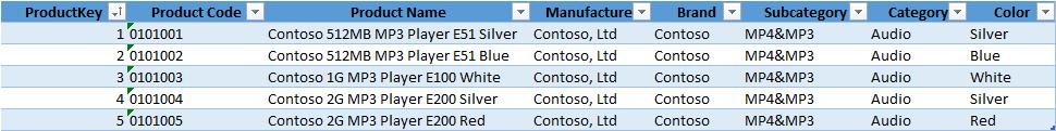
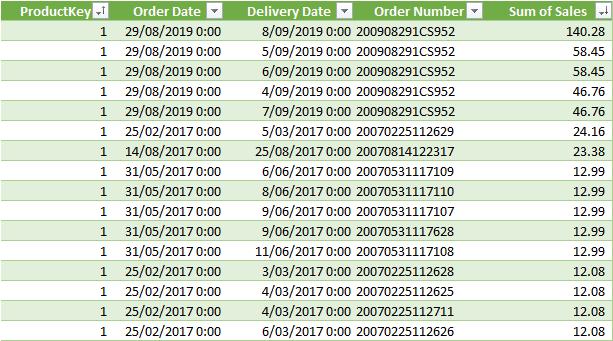
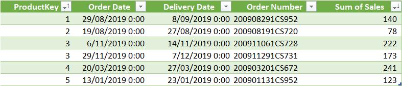
Let’s look at a simple example. Suppose we have following two tables, the Product table and Sales table (the Sales table is not displayed in full):
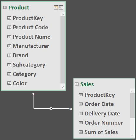
They have the following relationship (one-to-many relationship based on the ProductKey field):
Next, suppose we want to obtain the top sales value (i.e. “top 1 value“) in the Sales table. We may write the DAX syntax as following:
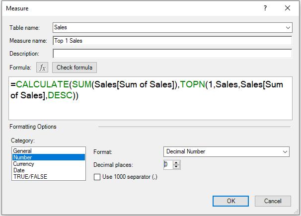
=CALCULATE(SUM(Sales[Sum of Sales]),TOPN(1,Sales,Sales[Sum of Sales],DESC))
We calculate the sum of sales and apply the filter by using the TOPN function. In the TOPN function, we specify the top one (1) row to be returned in descending order. Then, we export the result as a PivotTable and choose the ProductKey, Product Name and Top 1 Sales as fields. The result would be:
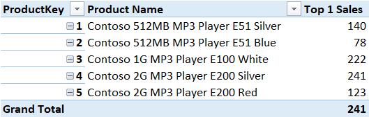
In this scenario, we can see the top one (1) sale for each product. This result can be confirmed further by the raw data below:
We may implement another measure which calculates the top five (5) sales values in same way.
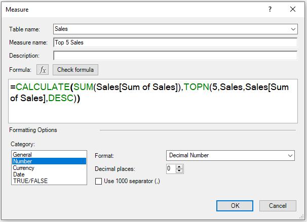
=CALCULATE(SUM(Sales[Sum of Sales]),TOPN(5,Sales,Sales[Sum of Sales],DESC))
The resulting PivotTable would be:

Let’s compare the result in the PivotTable with the raw data:
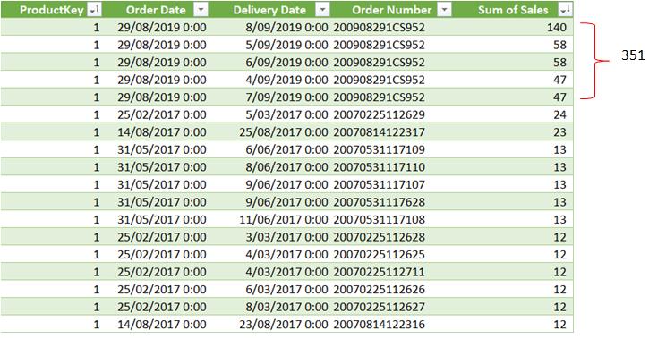
We can see that for product 1, the total of the top five (5) records is 351 (allowing for roundings), which is the same result shown in the PivotTable above. The measure ‘Top 5 Sales’ summarises the amount of the first five records in descending order.
Finally, we may write another measure which calculates the top three (3) sales values. This time, we want to create a chart to identify the trend for different top N measures.
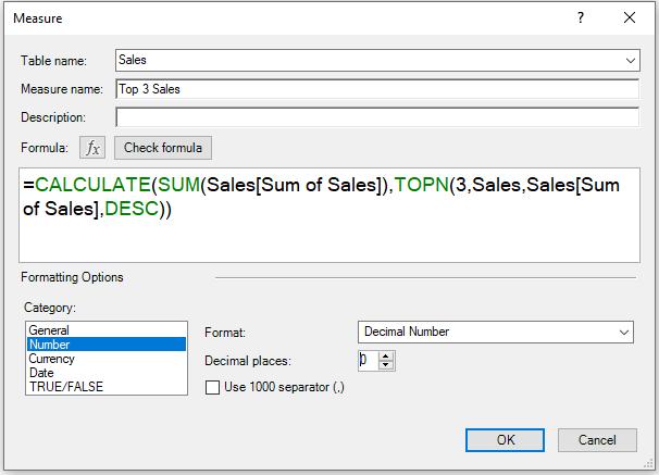
=CALCULATE(SUM(Sales[Sum of Sales]),TOPN(3,Sales,Sales[Sum of Sales],DESC))
Then, we may create the following PivotChart:
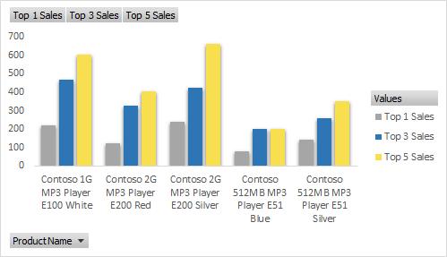
We list the top N values according to different product names. Thus, we can see different growth rates for each product.
That’s it for this week!
Stay tuned for our next post on Power Pivot in the Blog section. In the meantime, please remember we have training in Power Pivot which you can find out more about here. If you wish to catch up on past articles in the meantime, you can find all of our Past Power Pivot blogs here.