Power Pivot Principles: Filtered Imports

Welcome back to our Power Pivot blog, today we look at filtering the data a little before importing it form Excel. This blog builds on our previous blog Power Pivot Principles: Importing from Excel.

Returning to the Table Import Wizard (introduced last time), instead of selecting ‘Finish’ immediately, you can select ‘Preview and Filter’. This is recommended as it is always best (especially with large datasets) to import only what you need – “less is more”. You can always return and pick up extra data should you need it later.

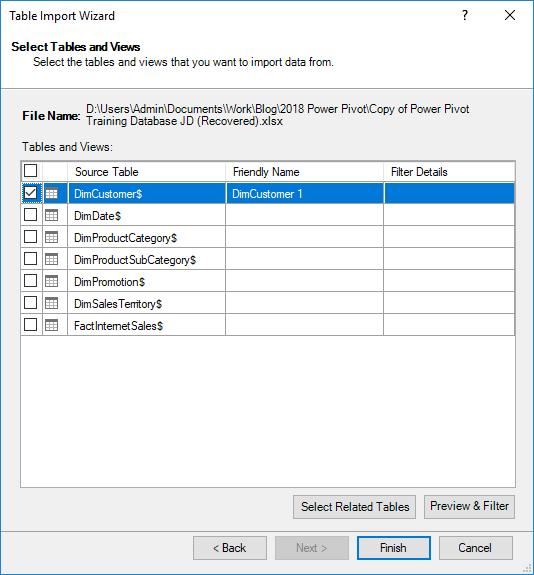
The Table Import Wizard will appear (below). This window allows us to uncheck the check box on each column of data to prevent that column from being brought into the model. We can also use the drop-down arrow on each column to filter the data and select only relevant data should this be required. You can download our sample dataset here.

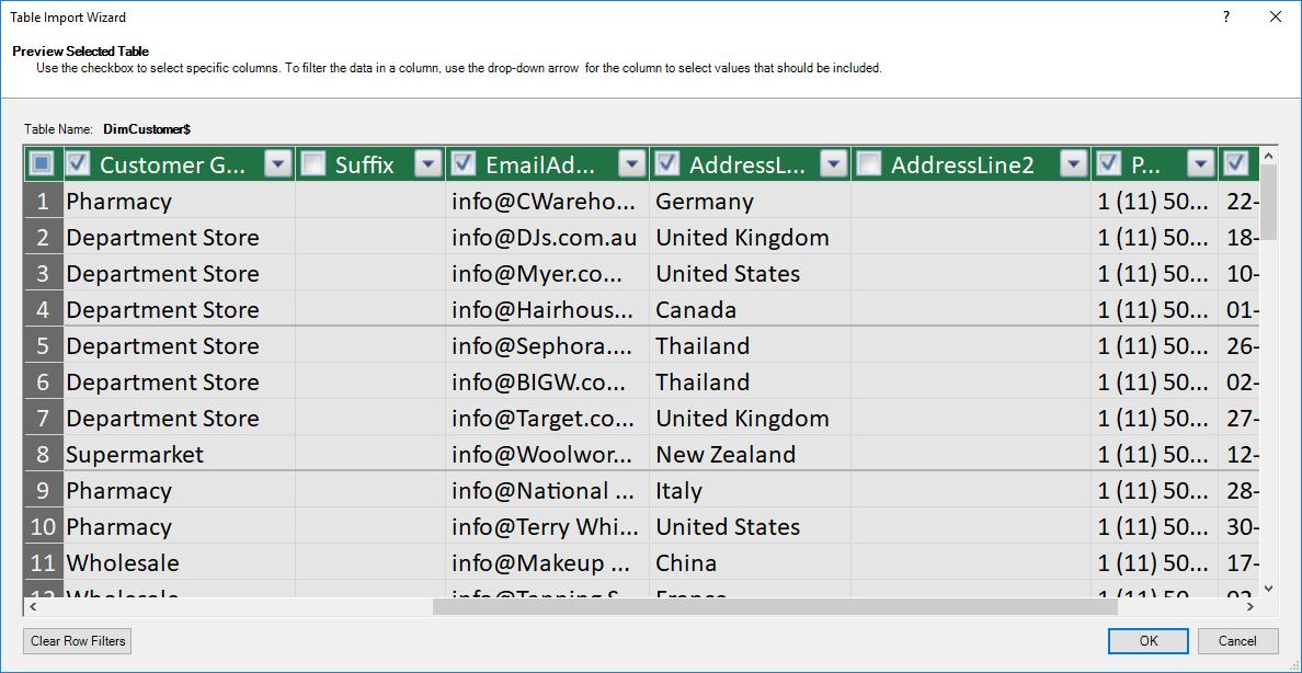
• In our example, unselect the checkbox for ‘Suffix’ and ‘AddressLine2’ – there isn’t any data in these columns and therefore we don’t need to bring these columns in to the model
• Select ‘OK’
• Ensure that all worksheets are brought into the model except for ‘DimPromotion$’
• Select ‘Finish’ to import.

A message will appear showing that the import was successful:

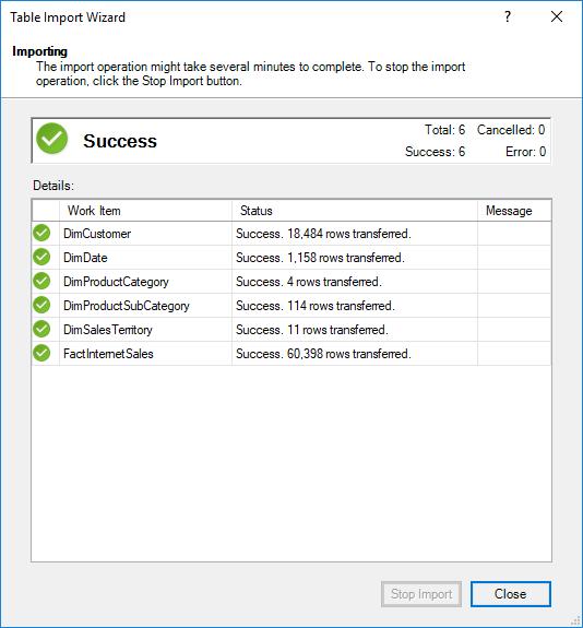
When importing multiple tables simultaneously, sometimes the final row may contain an error which does not relate to any particular table. Always read the error, but often this pertains to the fact that Power Pivot cannot recognise how the tables may be related. Take note if this is the case, but it is not an issue that has prevented a successful import of your data.

The data will now appear in separate tabs in the Power Pivot window as shown below:

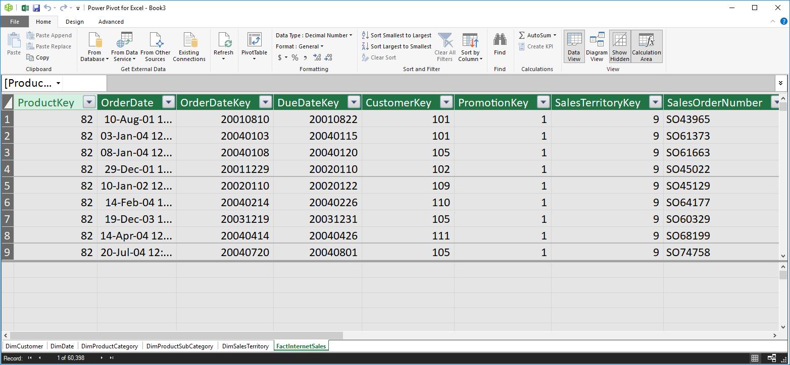
Whoops! I forgot to bring in the ‘DimPromotion$’ table into the model. So, let’s import it now!

• Click on ‘Existing Connections’ under the ‘Get External Data’ group:

• The following dialog box will appear:

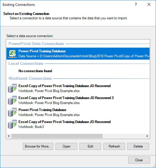
• Select the connection to the original data source
• Select ‘Open’
• The ‘Table Import Wizard’ will appear:

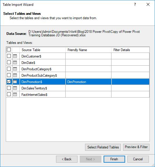
• We can select the table we missed on the original import ‘DimPromotion$’
• Either ‘Preview and Filter’ the data or select ‘Finish’.

Great – now we have the ‘DimPromotion$’ table in our data set. It’s that easy!

Stay tuned for our next post on Power Pivot. In the meantime, please remember we have training in Power Pivot which you can find out more about here. If you wish to catch up on past articles in the meantime, you can find all of our Past Power Pivot blogs here.