
Power Pivot Principles: Dynamic Ranking based on Selection Filters
23 July 2019
Welcome back to our Power Pivot blog. Today, we show you how to create a dynamic ranking measure that changes based on selection filters.
This week we are going to create a measure that will dynamically rank product prices based on a selection filter. We are going to use the ALLSELECT and CALCULATE functions, you can read about the ALLSELECT function here, and the CALCULATE function here.
For this example, we are going to use the following dataset:
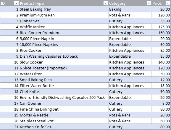
You might recognise this Table, as it is the same dataset used in last week’s blog, with a new column ‘Category’ added. You can read last week’s blog here.
Let’s imagine that we want to create a PivotTable that will display the products and their prices based on the category.
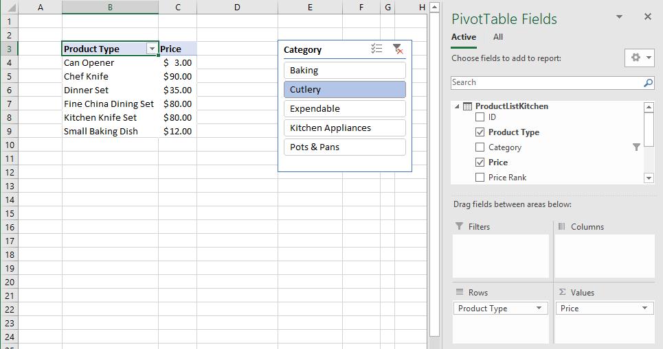
Now, we wish to have another column that will rank the products based on their prices. We have created a ranking column previously; lets see if this will work here.
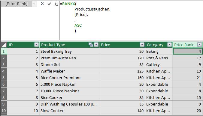
As a recap, we created a ranking column in PowerPivot with the following DAX code here:
=RANKX(
ProductListKitchen,
[Price],
,
ASC
)
Let’s see if bringing this column into our PivotTable will work:
The Rank column does not seem to be dynamic. Let’s try creating a measure instead. We are going to use the following DAX code:
=RANKX(
ALLSELECTED(ProductListKitchen),
SUM(ProductListKitchen[Price]),
,
ASC
)
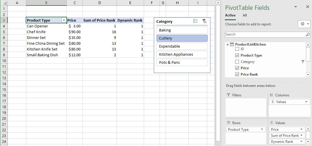
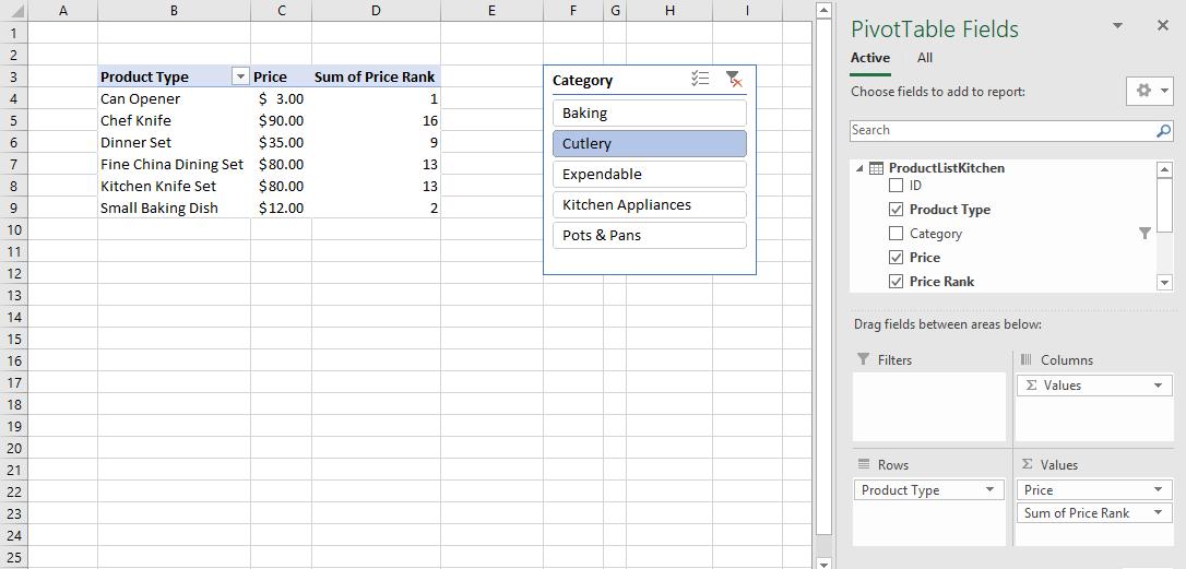
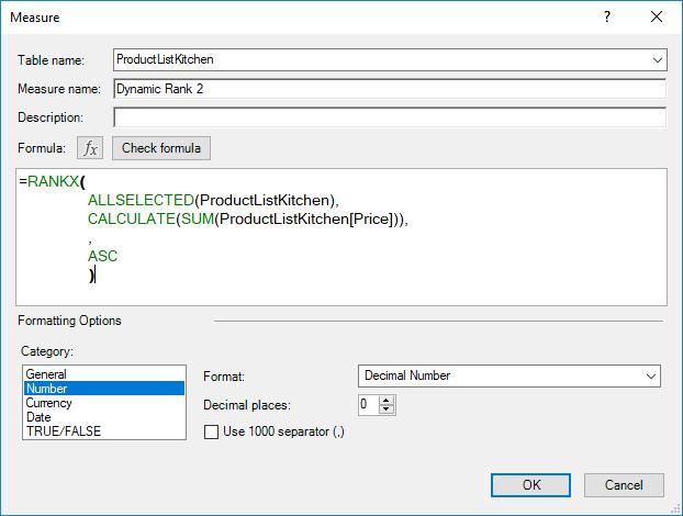
All of the ranks appear as ‘1’. This is because the RANKX function is going through each row individually and ranking that row’s ProductListKitchen[Price] with itself on the same row. Therefore, it will always be 1. We need to wrap the CALCULATE function around the current expression. This will bypass the current row by same row comparison, and compare the current row’s price with the rest of the table, viz.
=RANKX(
ALLSELECTED(ProductListKitchen),
CALCULATE(SUM(ProductListKitchen[Price])),
,
ASC
)
After wrapping the CALCULATE function, our PivotTable looks like this:
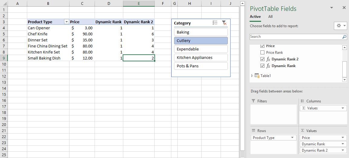
We can change our slicer selection and the dynamic rank will be applied.
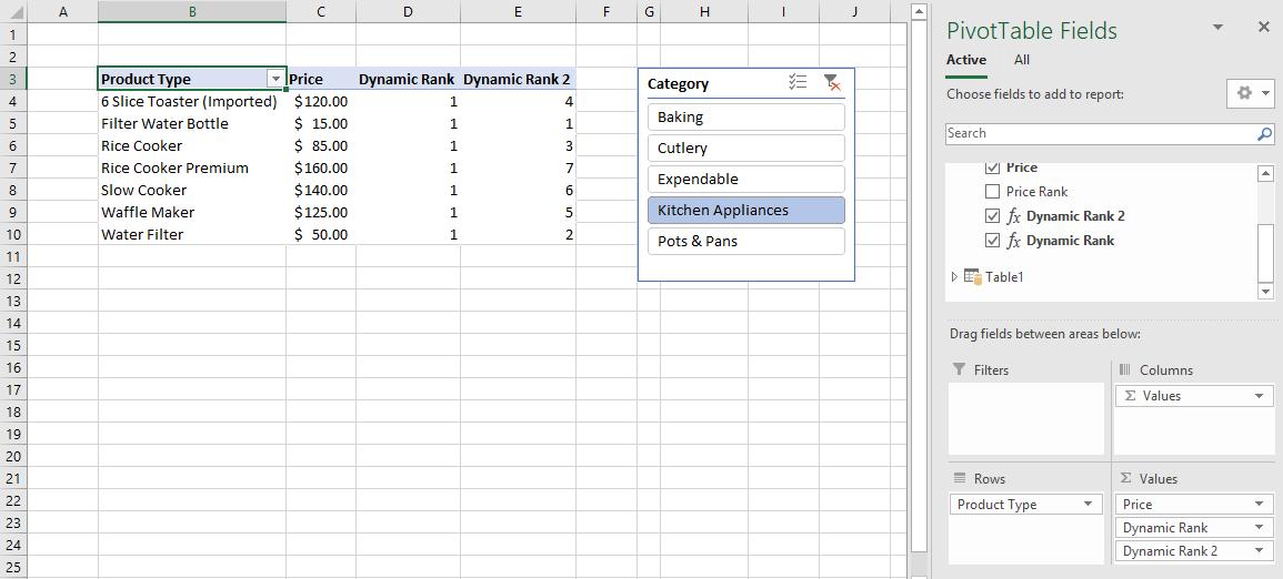
There we have it, we have dynamically ranked our products by ascending price in our data table.
That’s it for this week, come back next week for more Power Pivot. Until then happy pivoting!
Stay tuned for our next post on Power Pivot in the Blog section. In the meantime, please remember we have training in Power Pivot which you can find out more about >here. If you wish to catch up on past articles in the meantime, you can find all of our past Power Pivot blogs here.