Power Pivot Principles: The A to Z of DAX Functions – CEILING

In our long-established Power Pivot Principles articles, we continue our series on the A to Z of Data Analysis eXpression (DAX) functions.  This week, we look at the  CEILING...

The CEILING function

Have you reached your CEILING?  This function returns number rounded up, away from zero, to the nearest multiple of significance.

For example, if you are an American (which, let’s be honest is all Microsoft really cares about) and you want to avoid using cents in your prices (that makes no cents) and your product is priced at $12.24, use the formula =CEILING(12.24, 0.05) to round prices up to the nearest nickel.

The CEILING function employs the following syntax to operate:

It has two following arguments:

• number: this is required and represents the value you wish to round or a column that contains values
• significance: this is also required.  This is the multiple used for rounding.

It should be further noted that:

• regardless of the sign of number, a value is rounded up when adjusted away from zero.  If number is an exact multiple of significance, no rounding occurs
• if number is negative, and significance is negative, the value is rounded down, away from zero
• if number is negative, and significance is positive, the value is rounded up towards zero
• if either argument is non-numeric:

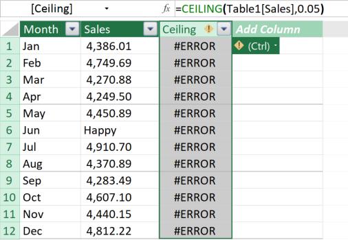
            - a calculated column using CEILING will return #ERROR values.  For instance:

            - a measure using CEILING will return a pop-up error warning message.

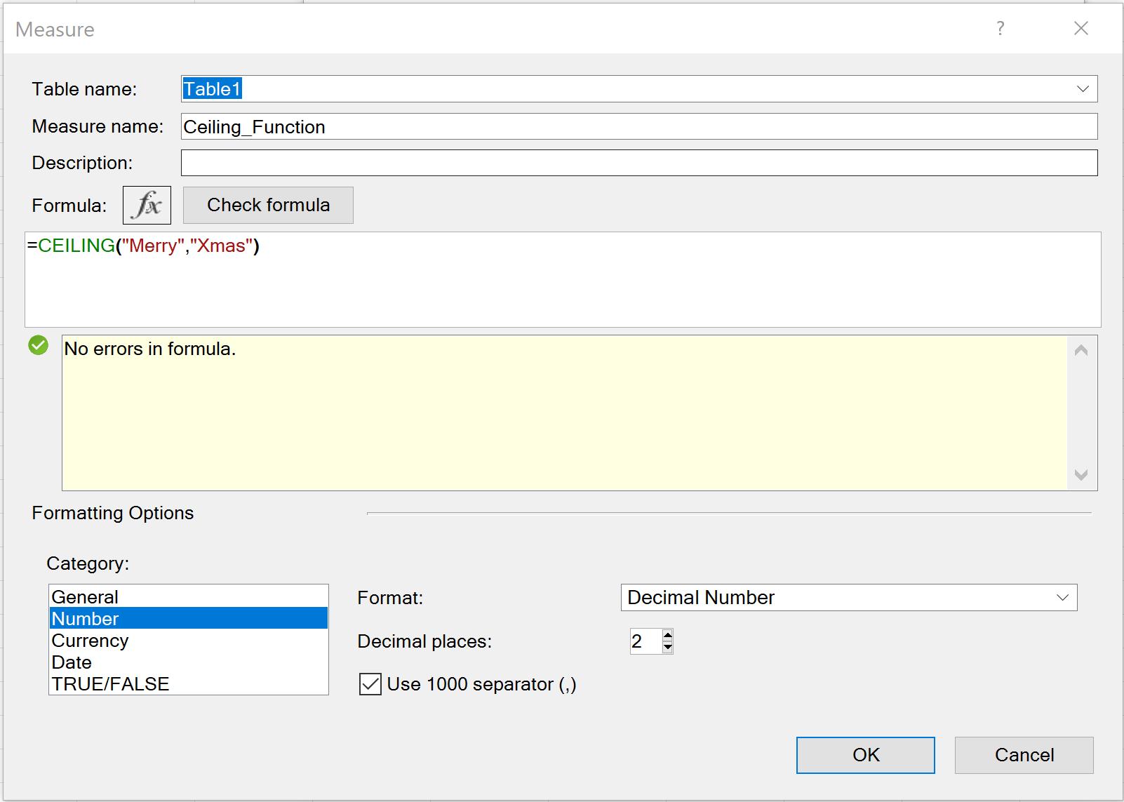
For example, we have a DAX measure below.  Although both arguments are non-numeric, the ‘Check formula’ button does not recognise any error in the formula:

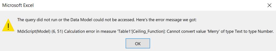
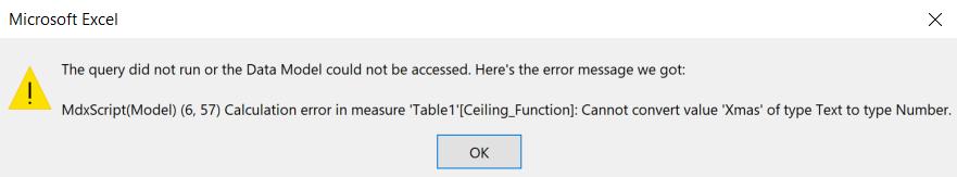
However, when the measure is used, one of the two error messages below will occur, depending upon whether number or significance is non-numeric.

Examples

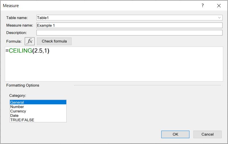
Example 1: The formula below will round 2.5 up to the nearest multiple of 1 and return 3.

Example 2: The formula below will round -2.5 up to the nearest multiple of -2 and return -4.

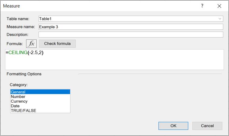
Example 3: The formula below will round -2.5 up to the nearest multiple of 2 and return -2.

Come back next week for our next post on Power Pivot in the Blog section. In the meantime, please remember we have training in Power Pivot which you can find out more about here. If you wish to catch up on past articles in the meantime, you can find all of our Past Power Pivot blogs here.