Power Pivot Principles: The A to Z of DAX Functions – AVERAGE

In our long-established Power Pivot Principles articles, we are starting a new series on the A to Z of Data Analysis eXpression (DAX) functions. This week it’s considered an ordinary function, if not quite AVERAGE…

The AVERAGE function

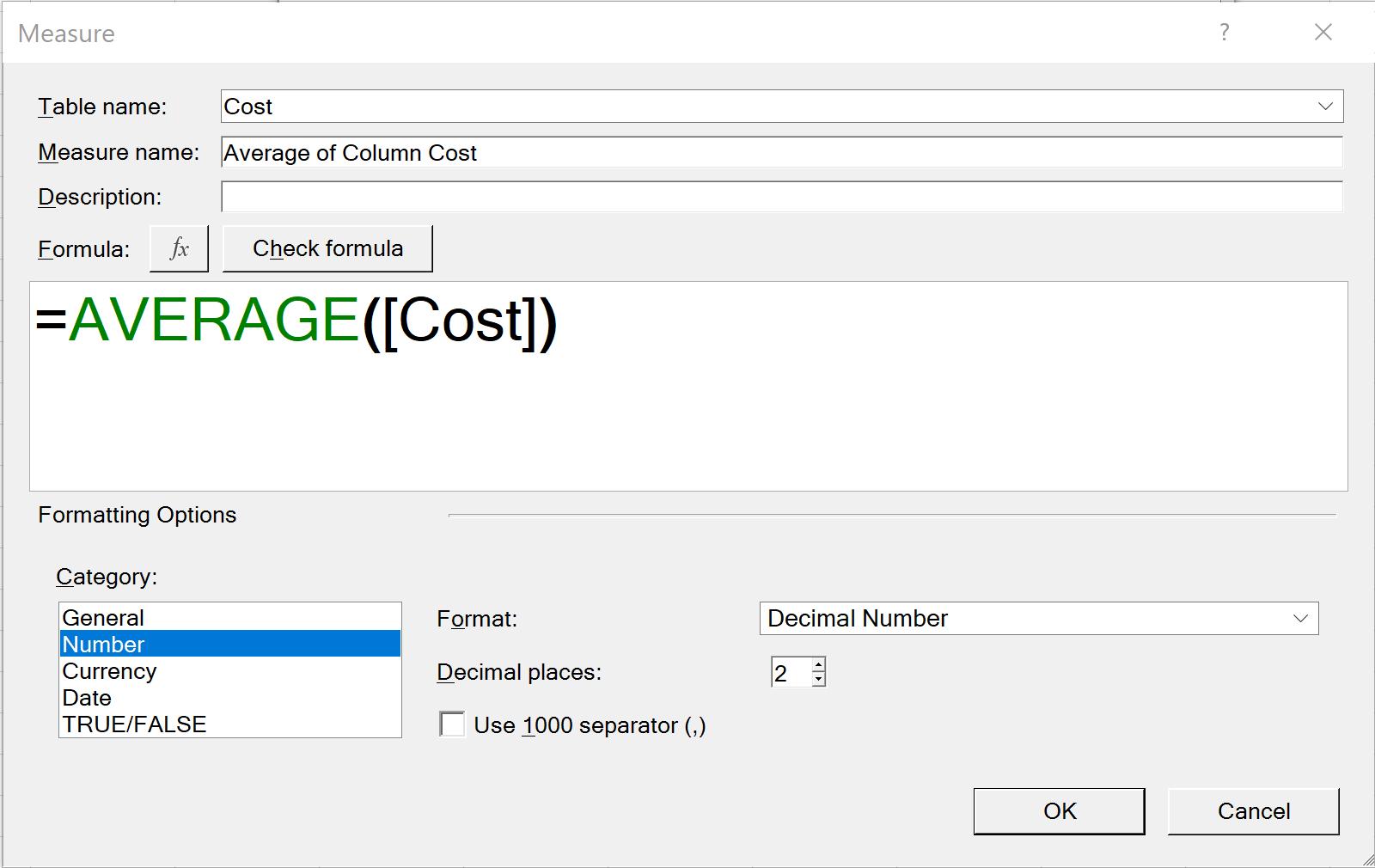
Today we look at the AVERAGE function. For example, we have a column called Cost, which contains numbers.  The DAX formula =AVERAGE([Cost]) returns the arithmetic mean of those numbers, including any zeroes.

The AVERAGE function measures what is known as “central tendency”, which is the location of the centre of a group of numbers in a statistical distribution.  There are three common measures of central tendency:

• average: the arithmetic mean, calculated by adding a group of numbers and then dividing by the count of those numbers.  For example, the average of 2, 3, 3, 5, 7, and 10 is 30 divided by 6, which is 5
• median: the middle number of a group of numbers.  That is, half the numbers have values that are greater than the median, and half the numbers have values that are less than the median.  For example, the median of 2, 3, 3, 5, 7, and 10 is 4.  If the number of values in the selection is an even number, the median is defined as the midpoint between the two central numbers
• mode: the most frequently occurring number in a group of numbers.  For example, the mode of 2, 3, 3, 5, 7, and 10 is 3.

For a symmetrical distribution of a group of numbers, these three measures of central tendency are all the same.  For a skewed distribution of a group of numbers, they can be different.

The syntax is straightforward:

There is only one argument:

• column: the column that contains the numbers that you want the average.

It should be further noted that:

this function takes the specified column as an argument and finds the average of the values in that column.  If you want to find the average of an expression that evaluates to a set of numbers, use the AVERAGEX function instead

• non-numeric values in the column are handled as follows:
• if the column contains text, no aggregation can be performed, and the functions returns blanks
• if the column contains logical values or empty cells, those values are ignored
• cells with the value zero are included
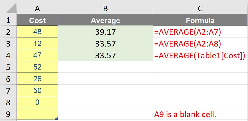
• when you average cells, you must keep in mind the difference between an empty cell and a cell that contains the value zero [0].  When a cell contains zero, it is added to the sum of numbers and the row is counted among the number of rows used as the divisor.  However, when a cell contains a blank, the row is not counted
• whenever there are no rows to aggregate, the function returns a blank.  However, if there are rows, but none of them meet the specified criteria, the function returns zero [0].  Excel also returns a zero if no rows are found that meet the conditions
• this function is not supported for use in DirectQuery mode when used in calculated columns or row-level security (RLS) rules.

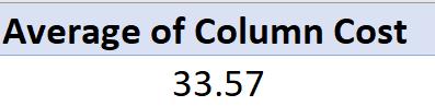
Please see my example below:

It works similarly to its Excel counterpart:

Come back next week for our next post on Power Pivot in the Blog section. In the meantime, please remember we have training in Power Pivot which you can find out more about here. If you wish to catch up on past articles in the meantime, you can find all of our Past Power Pivot blogs here.