
Power Pivot Principles: The A to Z of DAX Functions – AMORDEGRC
8 March 2022
In our long-established Power Pivot Principles articles, we continue our series on the A to Z of Data Analysis eXpression (DAX) functions. This week, we look at AMORDEGRC.
The AMORDEGRC function
Parlez-vous DAX? This function returns the depreciation for each accounting period in accordance with the French accounting system. If an asset is purchased in the middle of the accounting period, the pro-rated depreciation is considered. The function is similar to AMORLINC, except that a depreciation coefficient is applied to the calculation depending on the life of the assets.
The AMORDEGRC function employs the following syntax:
AMORDEGRC(cost, date_purchased, first_period, salvage, period, rate, [basis])
Important: Dates should be entered by using the DATE function, or as results of other formulas or functions. For example, use DATE(2016,5,23) for the 23rd day of May, 2016. Problems can occur if dates are entered as text instead.
The AMORDEGRC function syntax has the following arguments:
- cost: this is required. This represents the cost of the asset
- date_purchased: also required. The date of the purchase of the asset
- first_period: required. The date of the end of the first period
- salvage: required. The salvage value at the end of the life of the asset
- period: required. The period in question
- rate: required. The rate of depreciation
- basis: optional. The year basis to be used.
Some notes to remember on how the basis argument works (there’s no number 2):
| Basis | Date system |
|---|---|
| 0 or omitted | 360 days (NASD method) |
| 1 | Actual |
| 3 | 365 days in a year |
| 4 | 360 days in a year (European method) |
It should be noted that:
- dates are stored as sequential serial numbers so they can be used in calculations. In DAX, December 30, 1899 is day 0, and January 1, 2008 is 39448 because it is 39,448 days after December 30, 1899
- this function will return the depreciation until the last period of the life of the assets or until the cumulated value of depreciation is greater than the cost of the assets minus the salvage value
- the depreciation coefficients are:
| Life of assets (1/rate) | Depreciation coefficient |
|---|---|
| Between 3 and 4 years | 1.5 |
| Between 5 and 6 years | 2 |
| More than 6 years | 2.5 |
- the depreciation rate will grow to 50 percent for the period preceding the last period and will grow to 100 percent for the last period
- an error is returned if:
- cost < 0
- first_period or date_purchased is not a valid date
- date_purchased > first_period
- salvage < 0 or salvage > cost
- period < 0
- rate ≤ 0
- the life of assets is between zero [0] and one [1], one [1] and two [2], two [2] and three [3], three [3] and four [4], or four [4] and five [5]
- basis is any number other than 0, 1, 3 or 4
- this function is not supported for use in DirectQuery mode when used in calculated columns or row-level security (RLS) rules.
Please see my example below:
| Description | Value |
|---|---|
| Cost | $2,400 |
| Date purchased | 19 August 2008 |
| End of first period | 31 December 2008 |
| Salvage value | $300 |
| Period | 1 |
| Depreciation rate | 15% |
| Actual basis (see above) | 1 |
For this data, we may write the following code:
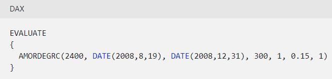
For the first period’s depreciation, given the conditions presented, the value returned will be $776.
Come back next week for our next post on Power Pivot in the Blog section. In the meantime, please remember we have training in Power Pivot which you can find out more about here. If you wish to catch up on past articles in the meantime, you can find all of our Past Power Pivot blogs here.