
Monday Morning Mulling: September 2019 Challenge
30 September 2019
On the final Friday of each month, we set an Excel problem for you to puzzle over for the weekend. On the Monday, we publish a solution. If you think there is an alternative answer, feel free to email us. We’ll feel free to ignore you.
Welcome to this month’s Monday Morning Mulling. Were you able to work around the error found in our last blog?
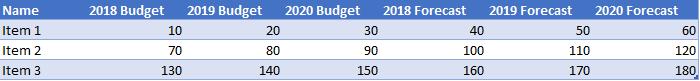
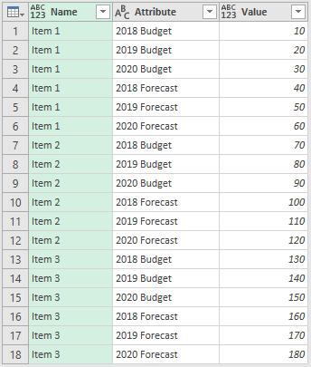
As a recap, we were presented with data similar to the following:
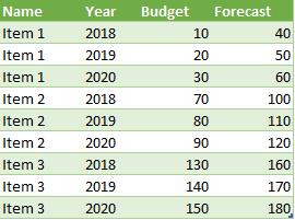
However, we want to present it as follows automatically:
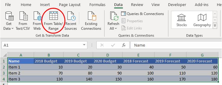
This sounds like a job for Power Query, which is our recommended approach. Therefore, the first thing we’ll do is load the Table into the Power Query Editor, viz.
It was hinted on Friday that this transformation fell in between an unpivot and a pivot. Well, I sort of lied – it’s actually one of each. First, we need to unpivot. Therefore, once in the Power Query Editor, we select the Name column only and then choose ‘Unpivot other columns’ from the ‘Unpivot columns’ dropdown in the Transform tab, as pictured:
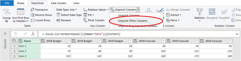
Note you don’t select the Budget and Forecast columns and unpivot them. If you do that, if the number of years were to be added, these columns wouldn’t be unpivoted. It’s safer to unpivot everything except for the Name field, viz.
If more fields appear (e.g. 2021 Budget, 2021 Forecast, 2021 Variance), these would automatically unpivot too.
Next, we want to split the Attribute column up into year and whether it is Budget or Forecast (in this instance). To do this, we should split the column at the space in each text string. This space is known as a delimiter, so it makes sense to select the Attribute column and then choose to split the column by delimiter as follows:
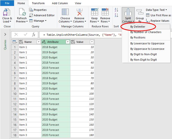
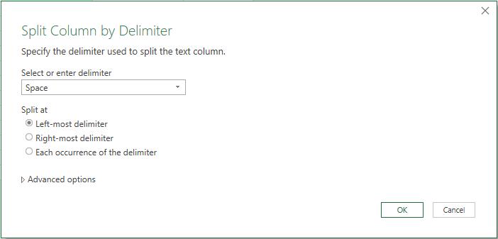
Bizarrely, this transformation is on the Home tab, not the Transform tab! Select the ‘By Delimiter’ option from the ‘Split column’ dropdown. This will generate the ‘Split Column by Delimiter’ dialog, where we will split on the first, left-most occurrence of the space delimiter.
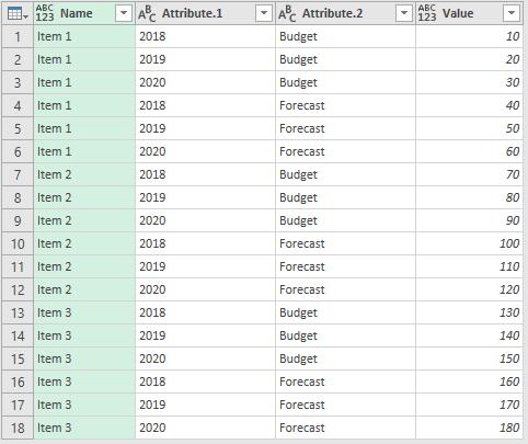
This results in the Attribute column effectively being split in two:
We are nearly there. We’ve decomposed (so to speak!), now we need to “re-compose”. It’s time to select the Attribute.2 column and use it for a pivot:
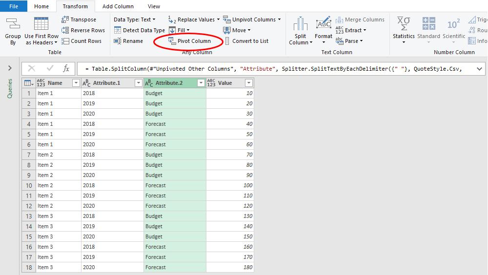
Having selected the Attribute.2 column, select ‘Pivot column’ from the Transform tab. This gives rise to the ‘Pivot Column’ dialog:
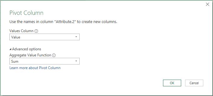
Ensure that it is the Attribute.2 column that is used to create new columns. Then, select the Value field as the ‘Values Column’ and choose ‘Sum’ as the ‘Aggregate Value Function’ in the ‘Advanced options’, all as pictured (above). This will then pivot the Attribute.2 column, creating two columns, Budget and Forecast, summing the values which relate to each context:
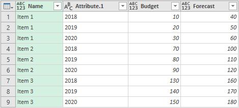
All that’s left to do now is rename the Attribute.1 column to Year and load it back into Excel:
Simple! If you want to play along at home, you can check out our example file here.
The Final Friday Fix will return on Friday 25 October with a new Excel Challenge. In the meantime, please look out for the Daily Excel Tip on our home page and watch out for a new blog every business workday.