Monday Morning Mulling: September 2017

On the final Friday of each month, we set an Excel for you to puzzle over for the weekend. On the Monday, we publish one suggested solution. No-one is stating this is the best approach, it’s just the one we selected. If you don’t like it, lump it – or contact us with your preferred solution.

Final Friday Fix: September Challenge Recap

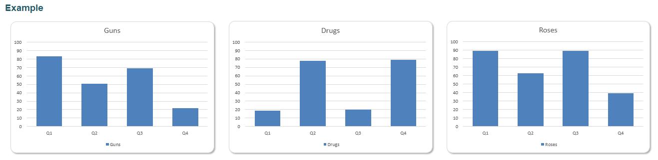
Last week we looked at three charts that pulled data from the same table, however, there was no easy way to format the y-axis on all three charts so that they all share the same range, without using a macro.

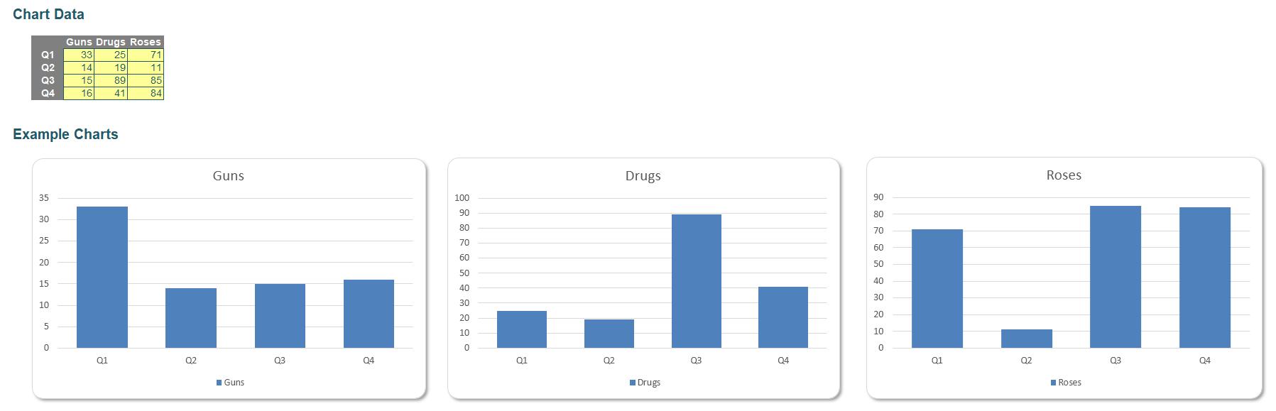
The Guns and Roses charts have a maximum y-axis range of 80, but the Drugs chart has a maximum of 120. We want all three charts to have the same range. How do we do this?

A Solution

The first step is to create a new column in the table that retrieves the maximum value:

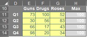
The new column has the following formula:

This will allow us to update the range of the graphs dynamically based on changing quarterly numbers.

The next step is to include the ‘Max’ column in each of the charts, we do this by right-clicking the charts and then selecting the ‘Select Data…’ option.

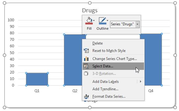
The ‘Select Data Source’ dialog box will appear:

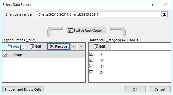
Click on the ‘Add’ button, to add the ‘Max’ column into the chart. Once you have included the ‘Max’ column into each chart they will have two columns for each quarter, similar to the ‘Gun’s chart featured below.

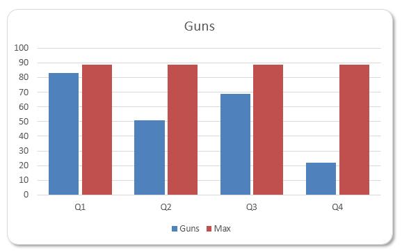
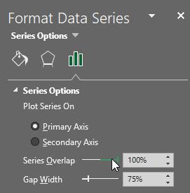
The trick here is to select the ‘Max’ (red) data series and choose the ‘Format Data Series…’ option, and adjust the ‘Series Overlap’ option to 100%.

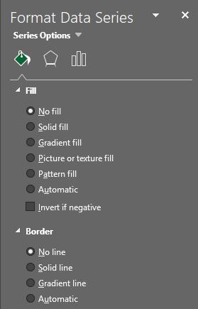
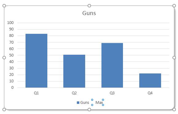
Now to get rid of the columns, adjust the ‘Fill’ and ‘Border’ settings to ‘No fill’ and ‘No line’ respectively.

The next step is to remove ‘Max’ from the legend. Double click it then hit ‘Delete’ on your keyboard!

Another trick to incorporate, in case those pesky headquarters staff continuously suggest changing chart titles, is to use a formula to decide the chart titles.  Click on each chart title and typing in the formula in the formula bar accordingly, for instance the ‘Guns’ chart should be linked to:

This works for simple formula references on the same sheet only.  Now, all three charts will not only have consistent but dynamic axes ranges, but also have self-updating chart titles.

So there you have it, charts that will dynamically update based on table data, all with the same y-axis ranges!

Neat? The final product can be downloaded here.

If you think you have a challenging problem that’s difficult to solve, let us know, and perhaps we will feature it in next month’s Final Friday Fix!