Monday Morning Mulling: May Challenge

On the final Friday of each month, set an Excel for you to puzzle over for the weekend. On the Monday, we publish one suggested solution. No-one is stating this is the best approach, it’s just the one we selected. If you don’t like it, lump it – or contact us with your preferred solution.

Final Friday Fix: May Challenge Recap

First appearing in Excel 2013, slicers are a visual filter that can be used to interact with PivotTables, PivotCharts or Tables. They are very popular with end users as they are highly intuitive requiring little more than a quick point and click.

The problem was that although are great for selecting one or more elements to filter, if there are many records to scroll through, searching is cumbersome. There appears to be no search facility.

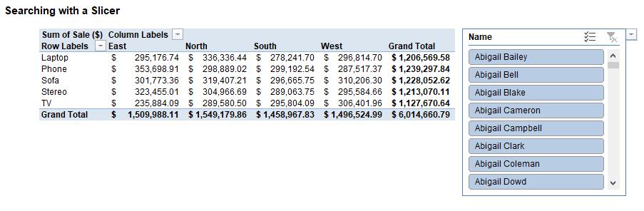
In the example above, wouldn’t it be good if you could search for, say, everyone whose surname was “Smith”?

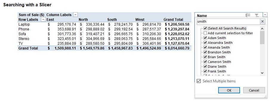
Clearly from the screenshot I appear to have achieved it. But that’s exactly my point. I appear to have achieved it. Perception is nine-tenths of the game sometimes. So how did I do it?

It’s easy – just follow these steps, assuming you are creating a slicer for a PivotTable:

• Create a PivotTable in the usual way
• Insert a slicer on the worksheet (click inside the PivotTable and then from the context tab ‘PivotTable Tools, Analyze’ tab on the Ribbon, select the slicer you require. You will note there is no search facility
• Make a copy of the PivotTable and paste it close to the original PivotTable. Note that the slicer is connected to both of these summary tables
• Remove all of the fields from the new PivotTable. If this causes an error, you have the two PivotTables too close together and you will need to separate them further apart
• In the Field list of the second (now empty) PivotTable, add the slicer field to the ‘Filters’ area of the PivotTable
• Now comes the clever part. Line up the slicer / adjust column widths so that it covers the filter button of the second PivotTable – except for the drop-down arrow. This gives the impression that the drop-down arrow ‘belongs’ to the slicer
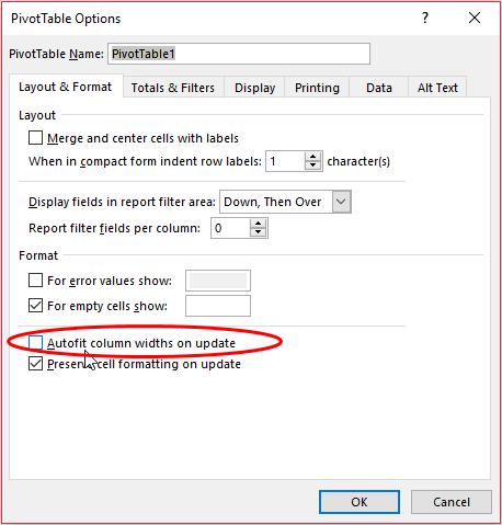
• Turn off the Autofit column widths option on both PivotTables (simply right-click on the PivotTable and select ‘PivotTable Options…’):

• Right-click on the slicer and select ‘Size and Properties…’ from the shortcut menu. In the ‘Properties’ section, choose ‘Don’t move or size with cells’

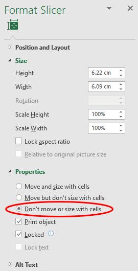
• These two setting changes will ensure the slicer continues to cover the second PivotTable
• Optionally, you can hide the column that contains the field name in the ‘Filters’ area of the new PivotTable.

That’s it! You can check out our example Excel file here.

For more tricks and tips, check out our many examples at www.sumproduct.com/thought. 

The Final Friday Fix will return on Friday 30 June with a new Excel Challenge.  In the meantime, please look out for the Daily Excel Tip on our home page and watch out for a new blog every other business workday.