
Monday Morning Mulling: July 2018 Challenge
30 July 2018
On the final Friday of each month, we set an Excel problem for you to puzzle over for the weekend. On the Monday, we publish a solution. If you think there is an alternative answer, feel free to email us. We’ll feel free to ignore you.
Final Friday Fix: July Challenge Recap
It makes a model easier to understand if there is good use of sections, subsections and subsubsections. Numbering makes for easier referencing too. Therefore, it’s recommended to include section headings (e.g. 1, 2, 3, …) and maybe subsection (e.g. 1.1, 1.2, …) and even subsubsection headings (e.g. 1.1.1, 1.1.2, …). Examples might look like the following (excluding all the content obviously!):
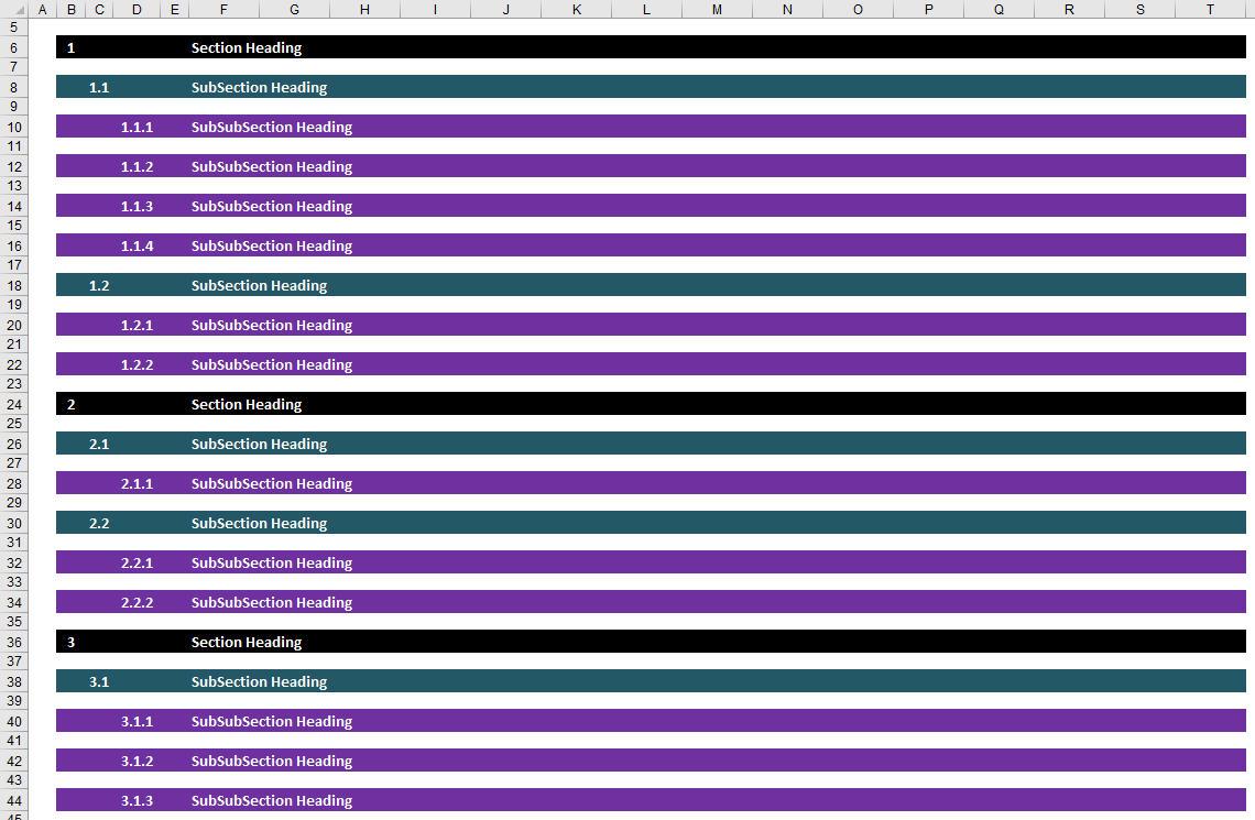
Therefore, in this month’s challenge we asked you to create row headings, subheadings and subsubheadings so that when you copy the appropriate the row section / subsection / subsection banner the numbering would automatically calculate (as above). For example, the subsection banner in row 8 could be copied into rows 18, 26, 30 and 38 in the example above and everything would then calculate automatically. It was part of the challenge that you should allow for numbering such as 4.103.17 too.
So how did you do?
Suggested Solution
As usual, we have an attached Excel file that works through our solution.
It’s clear whatever you do you are going to need some sort of counter that keeps track of what numbers have preceded it. Indeed, in SumProduct’s standard modelling template, we have such a formula in our section headers, viz.
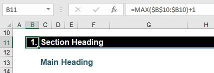
The formula in cell B11, namely
=MAX($B$10:$B10)+1
will add one (1) to the largest value it locates above it in column B. That works great, as long as there are no other numbers in column B – hence one of the reasons for the narrowed columns in our template (there are other reasons, but they are stories for other times).
Our idea here is similar, but more complex. We need to allow for numbering such as 1.1.1, 4.103.17 and 17.3.199 (say). If you think about this, we could do this by parsing the numbers 1,001,001, 4,103,017 and 17,003,199 in our examples. This means that:
- Section numbering requires a counter increasing in millions
- Subsection numbering requires a counter increasing in thousands
- Subsubsection numbering requires a counter increasing by one.
And that’s the idea really – after that it’s just about extracting the relevant data from the relevant numerical string and representing it as 17.3.199 etc. Therefore, we need a column for the counter – and I choose column E.
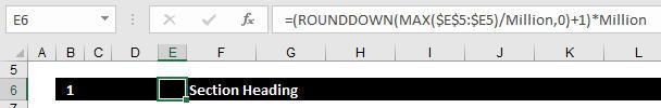
This column needs to remain blank with slightly different formulae for each type of banner heading. Let’s start off with the section heading banner:
Please note we have used range names Million for 1,000,000 and Thousand for 1,000 to avoid unnecessary hard code in our formulae. You can learn more about range names here.
Surprised about the complexity of the formula? The reason we need
=(ROUNDDOWN(MAX($E$5:$E5)/Million,0)+1)*Million
is as follows. Assuming all numbering starts in or after row 5, if the last counter were 16.043,002 which will come to mean 16.43.2, adding one million (1,000,000) would give us 17,043,002 (17.43.2) not the required new section 17. Therefore, this formula rounds down the previous largest number to the last million (16,000,000), divides it by a million (16), adds one (17) and then multiplies it by a million once more (17,000,000) which will equate to the next section heading number (17). There is a kind of weird logic to it, I promise!
The idea for the subsection counter is similar:
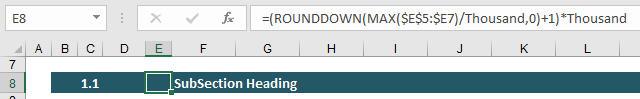
The formula
=(ROUNDDOWN(MAX($E$5:$E7)/Thousand,0)+1)*Thousand
simply replaces Million with Thousand (as well as updates the column referencing), so that one (1) is added at the Thousand level with the units reset to 1. For example, the next subsection after 4.5.6 will be 4.6.1 as 4,005,006 is progressed to 4,006,001.
The formula for the subsubsection is the simplest of all:
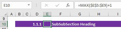
PhD’s in rocket science are not required!
=MAX($E$5:$E9)+1
simply adds one (1) to the last counter, just like our original heading formula.
All that is left to do is extract the relevant part of the number and re-present it. To begin with, it’s easy. For the section header counter, the formula is simply
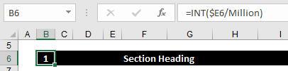
=INT($E6/Million)
where INT takes the integer part of the expression $E6/Million (i.e. it effectively rounds down). Things get more interesting, however, when we inspect the subsection heading numbering formula:
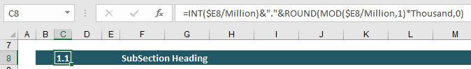
=INT($E8/Million)&"."&ROUND(MOD($E8/Million,1)*Thousand,0)
It should be noted that the indentation for subsection and subsubsection heading numbering is for aesthetic purposes only and is not required formulaically.
The first part of the formula (INT($E8/Million)) simply provides the section counter as before. The second part (&"."&) merely joins two expressions together using the concatenation operator, the ampersand (&) (you can find out more about concatenation here). It’s the third part that’s the charm:
ROUND(MOD($E8/Million,1)*Thousand,0)
Now ROUND(X,0) rounds the number X to the nearest whole number (0 refers to the number of decimal places for rounding purposes). The key part is
MOD($E8/Million,1)*Thousand
Some readers may not be aware of the MOD function. MOD(number,divisor), returns the remainder after the number (first argument) is divided by the divisor (second argument). The result has the same sign as the divisor.
For example, 9 / 4 = 2.25, or 2 remainder 1. MOD(9,4) is an alternative way of expressing this, and hence equals 1 also. Note that the 1 may be obtained from the first calculation by (2.25 – 2) x 4 = 1, i.e. in general:
MOD(n,d) = n - d*INT(n/d),
where INT() is the integer function in Excel.
This function has various uses in financial modelling, but the one I wish to discuss here is obtaining a residual (I sound like an actor). In some instances in modelling, you only want the decimal part (i.e. the numerical data after the decimal point). MOD(X,1) returns number after the decimal place, since it represents X – INT(X); the MOD approach is simply shorter. You can read more about MOD here.
Therefore, returning to our expression
MOD($E8/Million,1)*Thousand
dividing by a million puts the subsection and subsubsection data after the decimal point. Using MOD removes the integer part, and then multiplying by a thousand reverts the subsection number to an integer (whole number) whereas the subsubsection number remains after the decimal point. Rounding to the nearest whole number works fine as long as the subsubsection counter is below 500!
If that’s a little much to get your head around, let’s revisit the full formula
= INT($E8/Million)&"."&ROUND(MOD($E8/Million,1)*Thousand,0)
with the number 16,177,012 in cell E8 (say):
- INT($E8/Million) divides 16,177,012 by one million (16.177012) and takes the integer part (16)
- &"."& adds a decimal point to the end (16.)
- MOD($E8/Million,1) takes 16,177,012 and divides it by a million again (16.177012) but then removes the integer part (0.177012)
- MOD($E8/Million,1)*Thousand multiplies this result by a thousand (177.012)
- ROUND(MOD($E8/Million,1)*Thousand,0) rounds this number to the nearest whole number (177)
- This is then joined to the rest of the expression (16.177)
- Note the subsubsection element (0.012 or 12) is ignored – this would be zero in any case using the formula for subsection counters in column E.
The formula for the subsubsection counter is more of the same:

=INT($E10/Million)&"."&ROUNDDOWN(MOD($E10/Million,1)*Thousand,0)
&"."&ROUND(MOD($E10/Thousand,1)*Thousand,0)
This formula is similar to the subsection counter with the appendage
&"."&ROUND(MOD($E10/Thousand,1)*Thousand,0)
This simply removes all but the subsection number, which is then converted to an integer too. This works as long as the final three digits of the value in column E are less than 500.
Word to the Wise
You may have noticed I stayed away from INT and ROUNDDOWN in my formulae for determining the whole number values for the subsection and subsubsection numbers. This was deliberate. These functions appear to have exacerbated rounding errors when used with MOD. Try it and see!
The Final Friday Fix will return on Friday 31 August with a new Excel Challenge. In the meantime, please look out for the Daily Excel Tip on our home page and watch out for a new blog every business workday.