
Monday Morning Mulling: July Challenge
31 July 2017
On the final Friday of each month, set an Excel for you to puzzle over for the weekend. On the Monday, we publish a solution. If you think there is an alternative answer, feel free to email us. We’ll feel free to ignore you.
Final Friday Fix: July Challenge Recap
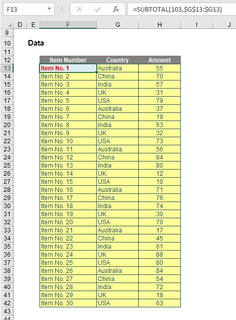
On Friday, I provided an attached Excel file. This file had data in the following format:
Highlighting the entire selection, I went to the ‘Data’ tab on the Ribbon and clicked on ‘Filter’ in the ‘Sort & Filter’ grouping (ALT + A + T) to create a filtered list. I then filtered on ‘Country’ for Australia and obtained the following subset:
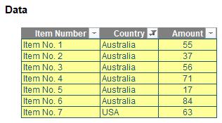
The problem was that when I did this ‘USA’ became part of the filtered ‘Australia’ subset. The questions were, why did this happen and how do you fix it?
The Solution
The problem here resides with the formula in cells F13:F42, namely
=SUBTOTAL(103,$G$13:$G13)
Yes, it will auto-number visible data, but there is an inherent problem in this formula too. Let me explain by first recapping on the SUBTOTAL function. On the face of it, it seems like many other Excel functions:
=SUBTOTAL(Function_Number, Ref1, Ref2, …)
The Function_Number is an integer between 1 and 11 inclusive or 101 and 111 inclusive as follows:
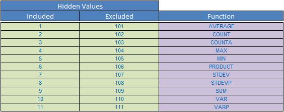
For the Function_Number constants from 1 to 11, the SUBTOTAL function includes the values of rows hidden by the ‘Hide Rows’ command under the ‘Hide & Unhide’ submenu of the ‘Format’ command in the ‘Cells’ group on the ‘Home’ tab. These constants should be used when you want to subtotal hidden and unhidden (visible) numbers in a list. For the Function_Number constants from 101 to 111, the SUBTOTAL function ignores values of rows hidden by the ‘Hide Rows’ command. These constants should be used when you want to subtotal the visible numbers in a list only.
If there are other subtotals within Ref1, Ref2, … (or nested subtotals), these nested subtotals are ignored. This is an important feature as it allows you to consider complete ranges without any risk of double-counting.
SUBTOTAL(103, Range) acts like COUNTA excluding any hidden cells, i.e. it counts the number of non-empty visible cells in Range. That’s how the auto-numbering works.
There’s just one problem.
SUBTOTAL also works with the built-in subtotal functionality of Excel, which totals numbers excluding – essentially, ignoring – the SUBTOTAL function. Therefore, Excel is trained to ignore what it thinks are subtotal rows.
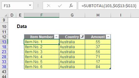
Look again at the USA row included. It’s the final row of the data selection and it begins with a SUBTOTAL function. Excel thinks it’s a subtotal calculation. Therefore, it has excluded it quite deliberately from the filtering believing it to be a subtotal of the data. Since the Function_Number lies between 101 and 111, Excel realises this function is designed to include filtered items only, so programmatically it makes sense to retain this row. Excel thinks it’s the sum of the above!
There are several ways that this logic can be defeated. This attached Excel file contains the following alternative ‘fixes’:
- Double Unary: possibly first discovered by Excel guru Dick Kusleika, putting two minus signs straight after the equals sign (e.g. =--SUBTOTAL(103,$G$13:$G13) ) fools Excel into thinking it’s a different formula. The first minus sign negates the calculation; the second makes it positive again
- Multiplying by 1: this one I am taking credit for! Who in their right mind would multiply a total by 1? Excel therefore thinks it isn’t a total and hence it becomes part of the filter set
- Add a column before the Item Number: In most instances (but sadly, not all), adding a column of data before the column containing SUBTOTAL will make the dataset work as intended. Suddenly Excel doesn’t believe the bottom row is a total anymore
- Add a blank row at the bottom: put a (sub)total at the bottom of the data? That’s just what Excel expected you to do! So don’t. Make it the penultimate row of the data by making a blank row part of the dataset. This is often quoted on the internet, but I think this is a terrible solution. If you need to add data, you’ll need to insert it before the blank row. What end user would appreciate the first blank row is part of the dataset? Further, blanks will be included in the list of options for the ‘Country’ filter. This is not an ideal fix
- Convert the data range to a Table: by highlighting the data and then converting the range to a Table (CTRL + T), filtering will work as expected – and you will get built in filtering as a bonus! Table totals work in a different way, so Excel is not confused by the SUBTOTAL formula. I quite like this solution as it requires no modification to the formula or need to add a row or column.
Other than adding a blank row (not sold on that at all), the others all have their strengths and weaknesses. I don’t want to advocate one solution over another. Hopefully, you came up with one of the above. If not – and it works – do let us know…
You can find out more about SUBTOTAL and Excel’s subtotal functionality here. For more tricks and tips, check out our many examples at www.sumproduct.com/thought.
The Final Friday Fix will return on Friday 25 August with a new Excel Challenge. In the meantime, please look out for the Daily Excel Tip on our home page and watch out for a new blog every other business workday.