Monday Morning Mulling: April Challenge

On the final Friday of each month, set an Excel for you to puzzle over for the weekend.  On the Monday, we publish one suggested solution.  No-one is stating this is the best approach, it’s just the one we selected.  If you don’t like it, lump it – or contact us with your preferred solution.

Final Friday Fix: April Challenge Recap

On Friday, I stated that a positive integer (whole number) is said to be prime if only two different numbers divide it: one and itself.  Therefore, the number 1 isn’t prime (it has only one divisor).  The challenge laid down was to ask, can you create a formula, without using a user-defined function or VBA, that will determine whether a number is prime?

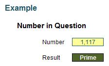
Let me call the number to evaluate, er, Number.  Some of you will have headed straight to the internet, to the home of your favourite search engine and located one of two very popular solutions, either

or

They have four things in common:

1. They are both array functions (i.e. entered using CTRL + SHIFT + ENTER – you do not try and type the braces ({ and }) in
2. These solutions are cited all over the internet, including on esteemed websites like Microsoft’s own Excel Blog
3. They are both fairly incomprehensible upon initial inspection
4. Neither actually work.

Yup, read point 4 again.  They’re wrong.  They don’t work in all situations – and yet they seem to be universally accepted.  And that’s the point of today’s blog.  When we don’t know how to do something, you head for your favourite search engine, hunt out the answer – and if you are wiser, check four or five sites to ensure they come to the same conclusion before accepting that answer. 

These formulae would pass that sniff test.  That’s my point.  But they are still wrong.

To show they don’t work, simply download this month’s attached Excel file, then try these:

Nobody tests anything anymore.  We are all download drones.  And this scares the living daylights out of me.  People might try numbers like 2, 17, 59, etc. and see it seems to work and conclude everything is fine.  But just because something is on page 1 of a well-known search engine page doesn’t make it true.

Ladies and gentlemen, as far as I am aware, please welcome the world premiere of a solution that works (within reason):

That’s right – it’s even worse than the other two.  In the next section, I’ll explain how this formula works, but feel free to stop reading at this juncture.  Showing off some horrendous calculation is not the objective of this article.  It’s realising that you should be careful when reading articles on how to solve things in Excel.  Yes, that includes my blogs too!

How the Formula Works

You don’t have to read this!  If you are interested though, the formula

needs to be picked apart.  However, before I do that, I need to show you a quick way to check for a prime.  Consider the divisors of 60:

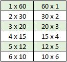
Do you see the symmetry?  Once you get to the middle – the square root – the factorisation reverses.  Since the square root of 60 is slightly less than 8, I only need to test to see if the numbers 1 to 8 divide 60.  Given 1 and n will always divide n, I only need to test the numbers 2 to ROUNDUP(SQRT(n),0) (the square root of n rounded up to the next whole number), which is 8 here.  This saves a lot of needless calculations!

This explains the element highlighted:

The function OFFSET(Reference, Rows, Columns, [Height], [Width]) has been discussed previously (see the article Onset of Offset for further details). 

The formula OFFSET($A$2,,,ROUNDUP(SQRT(Number),0)-1) gives a range of A2 to A8 if Number were 60 (1 has to be subtracted otherwise with a height of 8, you would get the range A2:A9).  Putting ROW() around this expression is a crafty way to convert to the numbers 2 to 8 inclusive.  This is why cell A2 must be a cell reference on row 2.

The next key element is MOD(Number, Divisor).  Again, I have discussed MOD before (please see A Modicum of MOD for further details): this provides the remainder after dividing Number by Divisor.  So, if I divide Number by each Divisor for the numbers 2 to ROUNDUP(SQRT(Number),0) – which would be 2 to 8 if Number were 60 – and any division gives me zero, that would mean Number is divisible by Divisor, i.e. the number is not prime.  If no division gives zero, it has to be prime so

{= IF(AND(MOD(Number,ROW(OFFSET($A$2,,,ROUNDUP(SQRT(Number),0)-1)))<>0),"Prime","Not Prime")}

gives the appropriate prime / not prime identification in certain circumstances.  This formula is both a variation of my proposed one and the second one identified as wrong earlier.  Do note it is encapsulated in an AND function and is in an array formula.  This forces Excel to perform all of the calculations from 2 to ROUNDUP(SQRT(Number),0) in one cell.  That’s a useful way of using an array formula (for more on arrays, please see Array of Light).

The rest of my formula,

is made up of tweaks to ensure: 

• Non-integers are not prime
• 0 is neither prime nor an error
• 1 is neither prime nor an error
• Negative numbers are neither prime nor an error.

My formula goes wrong eventually.  9 x 10²⁰⁰ is clearly not prime (it’s 3 x 10¹⁰⁰ squared) but Excel cannot evaluate it because it’s too large.  Meh, you can’t have everything!

Keep reading these articles, but stay cynical.  I am as prone to mistakes as the next persona (that’s a joke!).  By all means research, but convince yourself that it’s right.  Take nothing at face value.

For more tricks and tips, check out our many examples at www.sumproduct.com/thought.

The Final Friday Fix will return on Friday 26 May with a new Excel Challenge.  In the meantime, please look out for the Daily Excel Tip on our home page and watch out for a new blog every other business workday.