
Monday Morning Mulling: November 2019 Challenge
2 December 2019
On the final Friday of each month, we set an Excel problem for you to puzzle over for the weekend. On the Monday, we publish a solution. If you think there is an alternative answer, feel free to email us. We’ll feel free to ignore you.
To recap, the problem we presented last Friday was to challenge you to create an option list for a whole workbook. Specifically, we create a dashboard to track the accommodation and catering services for one of our imaginary clients:
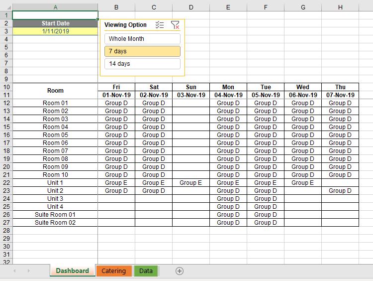
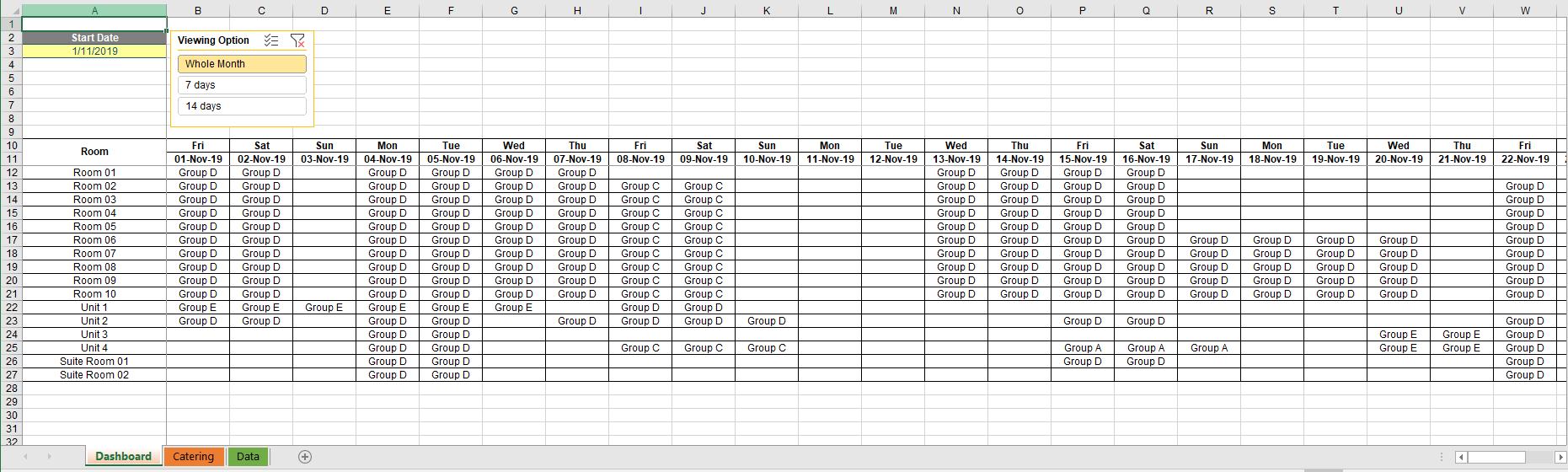
- a Dashboard sheet showing which customer group is staying in which room and on what date
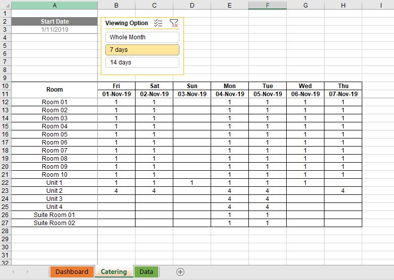
- a Catering sheet which displays the number of guests in each room and by date who will be using catering services. (This is simply generated by an INDEX-MATCH from the Data sheet.)
The client wants to be able to view by whole month, 14-day or 7-day in both reports at any time.
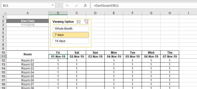
For example, we just need to input the ‘Start Date’, and click on option to view as ‘7 days’, the list will be generated for the whole week to see which group of customers will be coming:
whilst in the Catering sheet, the list is also updated accordingly, where we can see how many we need to prepare for catering:
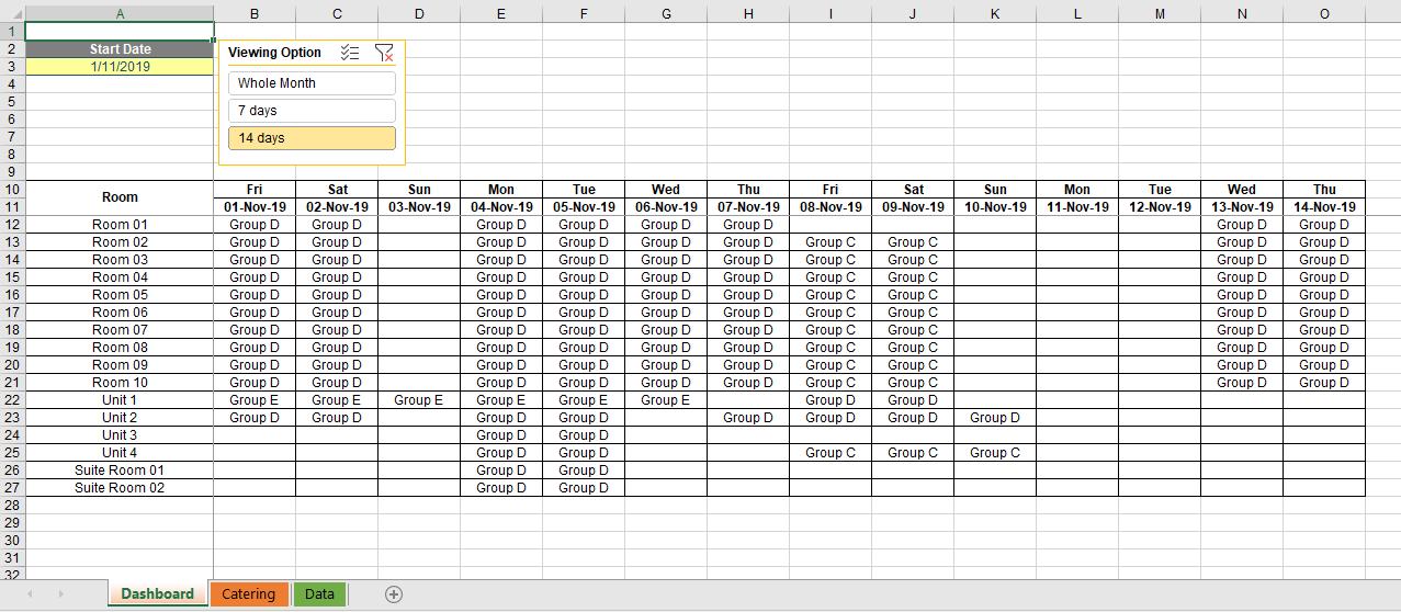
If we choose ’14 days’, the list is now longer:
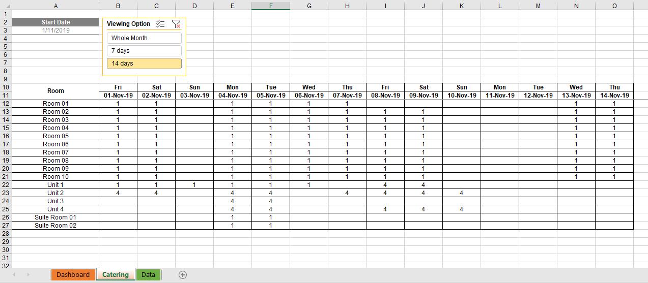
with a similar effect in the Catering sheet:
Further, the list will be updated for the whole month if we choose to view ‘Whole Month’:
Suggested Solution
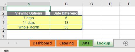
We need to create a lookup table for the ‘Viewing Option’ list in a separate worksheet (here called ‘LookupTable’). The table contains a ‘Viewing Options’ column, listing all of the options, and a ‘Date Difference’ column, indicating the number of days which will be added to the start date, viz.
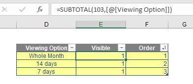
Next, we create a Selection table like the one below. This table contains the fields ‘Viewing Option’, a Visible indicator (where number 1 means the option has been chosen), and Order, which is used to sort. Cells in the Visible column are based on the formula:
=SUBTOTAL(103,[@[Viewing Option]])
where 103 represents the number function of COUNTA, with any hidden values excluded (you can read more about SUBTOTAL here.
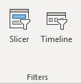
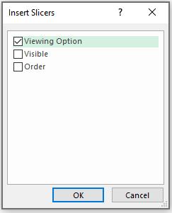
With the cursor in this table, go to the Insert tab and choose Slicer:
From the resulting ‘Insert Slicers’ dialog, since we want to have Viewing Option as a list, select this field and click OK.
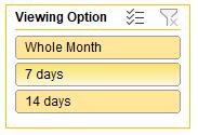
We will have a slicer box similar to the one below, where we can copy and paste to any sheet that we wish to use.
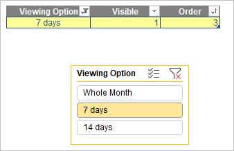
Now if we click on one of the options, the Selection table will only show the option being selected:
With the logistics prepared, go back to the main sheet and choose one cell – here, cell C5 – which indicates the option ticked from the slicer box (note here that later this cell will be hidden behind the slicer box). This cell C5, named ‘ViewingOption’, contains the following formula to look up the visible option from the Selection table:
=INDEX(SelectionTable[ViewingOption],MATCH(1,SelectionTable[Visible],0))
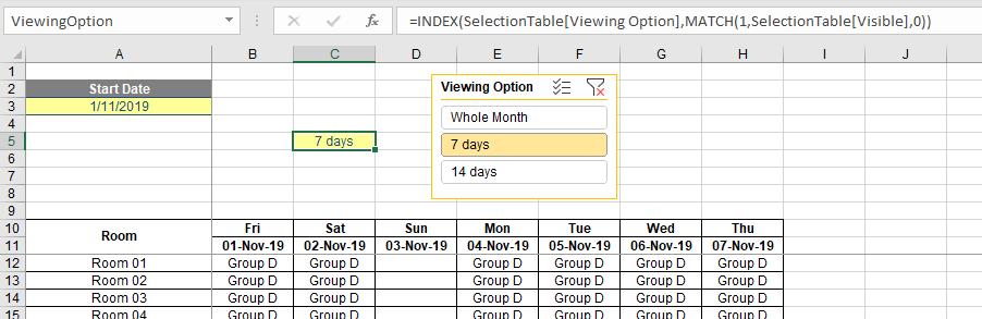
We will then need to generate the date list. Cell B11 is the first date of the list, which is the Start Date as an assumption. The formula in cell C11 is:
=IF(B11="","",IF(B11-DateChosen<INDEX(LookupTable[Date Difference], MATCH(ViewingOption,LookupTable[Viewing Options],0)),B11+1,""))
which compares the viewing option selected and looks up the date difference to add from the lookup table. We will copy the formula to 30 more cells, because we require 31 days maximum for a whole month. The relevant cells in row 10 contains the formula to show the day of week:
=IF(B11="","",TEXT(B11,"ddd"))
In the Catering worksheet, simply put all the cells equal to the relevant cells in the Dashboard sheet, noting that the slicer box is also copied here for easy reference. If we are in the Catering sheet and we want to view more or fewer days, just click the option on the slicer box in this sheet. It will trigger the Viewing Option cell (cell C5) in the Dashboard and then update the date list accordingly.
For the final touch, we need to set up some conditional formatting so that if the date is not shown, that date cell and all cells below it will not be bordered (to make them invisible). You can also hide the sheet containing the lookup table and Selection table to keep the magic all yours. Here is the completed file for your reference.
The Final Friday Fix will return on Friday 27th December 2019 with a new challenge. In the meantime, please look out for the Daily Excel Tip on our home page and watch out for a new blog every business workday.