Final Friday Fix: September Challenge

Filtering Labels

If you work with data across multiple categories, you’ll know some of the issues that arise when trying to group PivotTable data in different ways.  Not all data is sorted in numerical or date order, and sometimes, there are specific codes that apply to different digits in an account code or business unit name.

The Challenge

Today we have a fairly standard looking PivotTable – we have years going across the top of the table, and a list of product numbers going down the page, totalling up the sales by product in each year (you can download the Excel file example here).

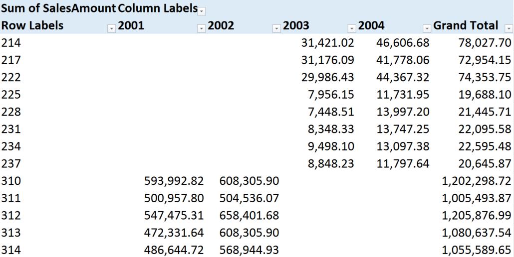
The challenge today is to filter the data, without changing the raw dataset, so that it will only display product numbers that have a ‘1’ as the middle digit. You can assume that there will only ever be three digits in the product number.

Note that filtering manually and selecting only the items with a ‘1’ as the middle digit won’t be scalable as new product numbers are incorporated into the list.

Think it sounds easy? You’ve done this before? Download the file and give it a shot, because it’s not as straightforward in this case as you think. We’ll publish our solution in Monday’s blog. Have a good weekend, and see you in October!