Monday Morning Mulling: October 2020 Challenge

On the final Friday of each month, we set an Excel / Power Pivot / Power Query / Power BI problem for you to puzzle over for the weekend. On the Monday, we publish a solution. If you think there is an alternative answer, feel free to email us. We’ll feel free to ignore you.

This month, we consider allocating days across monthly periods, where some dates are outside the forecast period and others straddle the (monthly) reporting periods.

The Challenge

As a reminder from Friday’s challenge, this month sees you work for an education establishment, seeking to model forecast data for the calendar year 2021. There are four terms relevant to your modelling period:

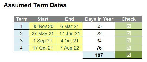
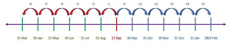
All we need to do is allocate the number of term days (including weekends and public holidays) to each month of 2021, i.e.

The challenge was “simply” this: were you able to construct a calculation such that the correct number of days would be allocated to each month? You were advised that you may assume the terms would be in chronological order, that they would not overlap, there will never be more than two terms associated with any given month, and there will never be two start dates or two end dates in the same month. There was even a starter file for you – although today we supply a completed file too…

Suggested Solution

It is possible to get into a mess with this quite quickly, because there are several scenarios to consider for any given reporting month. To get our heads around this, let’s consider just one monthly period, between x and y:

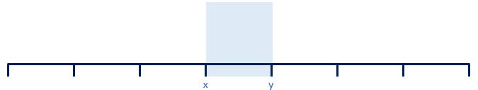
If x and y are day numbers, then the number of days in the period is

(we have to add one [1] as day x is actually in the period).  But how many days relate to the term?  Well, it depends.  There are actually five scenarios to consider:

Scenario 1: No Term Days

In this instance, no term days fall in the given period, so the number of days between x and y will be zero (0).

Scenario 2: Term Fully Insider Reporting Period

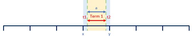
Here, the term starts at t1, which is greater than or equal to x, and ends at t2, which is less than or equal to y.  The number of days (a) is therefore given by

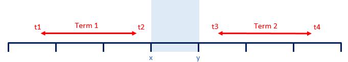
Scenario 3: Term Ends in Reporting Period

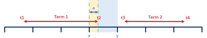
Here, I have Term 1 ending in the reporting period at t2, but Term 2 starts in a later period (i.e. after y) at time t3.  Therefore, the number of days (a) is given by

Technically, this formula is still

Scenario 4: Term Starts in Reporting Period

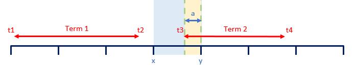
Here, I have Term 2 starting in the reporting period at t3, but Term 1 ends in an earlier period (i.e. before x) at time t2.  Therefore, the number of days (a) is given by

Since there is no distinction (algebraically) between t3 and t1, and similarly, between t4 and t2, we may interchange these variables, so that this formula is still equivalent to

In other words, Scenarios 2, 3 and 4 may all be solved using the same formula.

Scenario 5: One Term Ends and Another Starts in the Reporting Period

This situation is distinct from the others:

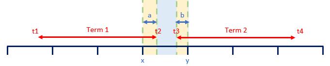
Here, I have Term 1 ending in the reporting period at t2, but Term 2 also starts in the same period at time t3.  Therefore, the number of days (a + b) is given by

which may be simplified slightly to

This situation occurs when a reporting period has both a relevant start date and a relevant end date, and the relevant start date occurs after the relevant end date for that period.

Modelling the Solution

We are now in a position to model the number of days in a period.  There are essentially three categories that the scenarios fall into:

1. No term days are in the reporting period
2. At least one of the start and / or end dates for a given term is in the reporting period (start date must be less than or equal to the end date)
3. One term ends and the next term starts within the reporting period (start date occurs after the end date for that reporting period).

Calculating the relevant end dates are not the problem.  If the end date of a term falls outside the reporting period, we just use the end of the period instead (deemed end).  However, start dates have two issues:

1. The start date may have occurred prior to the forecast period.  If the end date is also earlier, then this constitutes no issue, but if the end date is within the period, we will have to assume the deemed start is the first day of the reporting period
2. We need to check if the start date starts before / coincides or ends after the end date for a given reporting period.  This will determine the method of calculation.

With all this borne in mind, we are now in a position to model the problem, and our solution is attached here. 

First, we need to add the assumptions into our model:

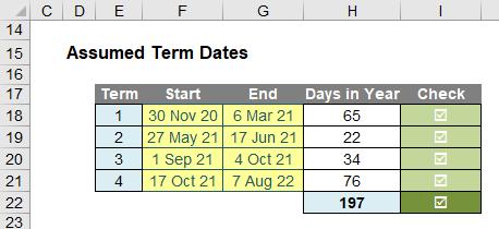
There are checks here to ensure that dates have been entered correctly and that the end date does not occur before its associated start date, etc.

Next, the relevant month ends associated with these dates are calculated using the EOMONTH function.

EOMONTH Reminder

As a recap, this function returns the serial number (Excel’s numerical representation of a date) for the last day of the month that is the indicated number of months before or after a given start_date. You should use EOMONTH to calculate calendar dates, maturity dates or due dates that fall on the last day of the month. This is a particularly useful function for creating time series in financial models.

The EOMONTH function employs the following syntax to operate:

The EOMONTH function has the following arguments:

• start_date: this is required and represents the start date.  Dates should be entered by using the DATE function, or as results of other formulas or functions.  For example, consider using DATE(2020,11,2) for the second (2^nd) day of November, 2020.  Problems can occur if dates are entered as text
• months: this is also required.  This represents the number of months before or after the start_date.  A positive value for months yields a future date; a negative value yields a past date.

Returning to the Modelling

The end of months used are simple for the end dates, but the start dates formula is a little more convoluted.

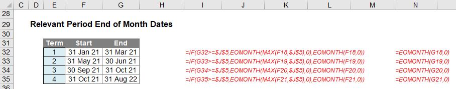
The formula in cell F32, for example, is

This checks to see if the end date occurs on or after the first day of the modelling period.  If so, the end of month for the start date is assumed to be the greater of the end of month of the given start date or the end of the first reporting month, whichever is later.  This is in case the start date occurred earlier than the model allows for (otherwise the number of days calculated would be incorrect).

This takes us to our final calculations:

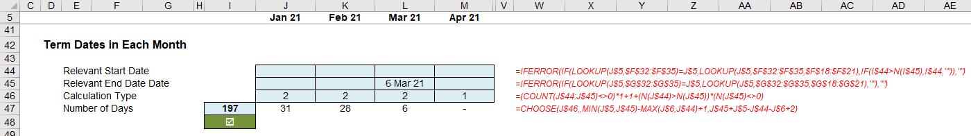
Apologies for the still small, yet truncated, screenshot. 

It is best to start with row 45, the Relevant End Date, as the concept here is simpler than the its counterpart for the Relevant Start Date.  The formula in cell J45 is given by

This formula uses LOOKUP.

LOOKUP Formula

The alternative form is the vector form:

The LOOKUP function vector form syntax has the following arguments:

• lookup_value is the value that LOOKUP searches for in the first vector
• lookup_vector is the range that contains only one row or one column
• result_vector is optional – if ignored, lookup_vector is used (which is what happens in the first part of the above formula) – this is the where the result will come from and must contain the same number of cells as the lookup_vector.

The lookup_value must be located in a range of ascending values, i.e. where each value is larger than or equal to the one before, which is why the terms must be in chronological order.

Returning to the Modelling (Again!)

The formula in cell J45 is given by

This checks if the end of term date occurs in that reporting period, and if so, returns that end date.  If it does not, the cell is attributed the empty (“”) string instead.

The formula in cell J44 uses this result, which is why the second row has been explained first.  The formula in cell J44 is given by

The first part of the formula is very similar to the calculation in the row below.  It checks if the start of term date occurs in that reporting period, and if so, returns that start date.  However, if it does not, it then checks whether there was a start and end date in the previous period.  As long as the start date exists (this is why N(I$45) is used – so that a blank cell is treated as zero), it then checks if the start date occurs after the end date.  This is to see whether we are in Scenario 5, as explained earlier.  In this case, the start date is required.

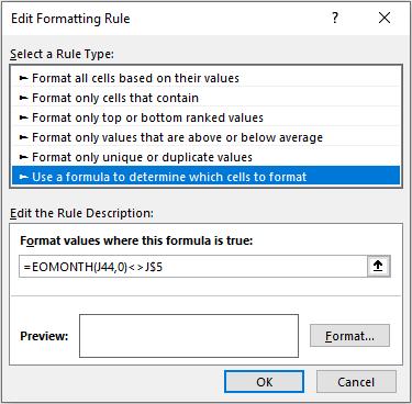
Astute readers will note that more dates should be visible than are shown in rows 44 and 45.  This is because we have hidden subsequent dates if they are not relevant to that period.  Dates have been made “invisible” using conditional formatting in that instance, viz.

We are nearly there.  The penultimate formula in cell J46 defines the Calculation Type.

This formula generates a number between one (1) and three (3):

1. No term days are in the reporting period
2. At least one of the start and / or end dates for a given term is in the reporting period (start date must be less than or equal to the end date)
3. One term ends and the next term starts within the reporting period (start date occurs after the end date for that reporting period).

This is simply the categorisations we derived what seemed like a lifetime ago now.

This leads us elegantly to our final formula in cell J47, which derives the Number of Days:

The CHOOSE function allows us to calculate the result all in one line.

CHOOSE Function

This function uses the first argument index_number to return a value from the list of value arguments.  CHOOSE may be used to select one of up to 254 values based on the index number (index_number).  

The CHOOSE function employs the following syntax to operate:

The CHOOSE function has the following arguments:

• index_number: this is required and is used to specify which value argument is to be selected.  The index_number must be a number between 1 and 254, or a formula or reference to a cell containing a number between 1 and 254.
  • if index_number is 1, CHOOSE returns value1; if it is 2, CHOOSE returns value2; and so on
  • if index_number is less than 1 or greater than the number of the last value in the list, CHOOSE returns the #VALUE! error value
  • if index_number is a fraction, it is truncated to the lowest integer before being used.
• value1, value2, ...: value 1 is required, but subsequent values are optional.  There may be between 1 and 254 value arguments from which CHOOSE selects a value or an action to perform based on index_number.  The arguments can be numbers, cell references, defined names, formulas, functions or text.

One Last Time

As stated above, the formula in cell J47 derives the Number of Days:

Cell J46 returns a value of 1, 2 or 3 to determine the category.  If the value is:

• zero (0): the number of days returned is zero (0), as there are no term days in the reporting month
• one (1): the formula used is MIN(J$5,J$45)-MAX(J$6,J$44)+1, which is the Excel equivalent of the calculation derived earlier for Scenarios 2, 3 and 4
• two (2): the formula used is J$45+J$5-J$44-J$6+2, which is the Excel equivalent of the calculation derived in Scenario 5.

The final check in the screenshot, 

simply checks that the number of days in row 47 is equal to the number of days calculated earlier

in cell H22.

Word to the Wise

I am conscious there are other ways to calculate a solution to this month’s challenge.  Some of you may have elected to work out which term was relevant on the first day of the period, and which was relevant on the last day.  That works in this situation too, as only two terms may straddle any given month (one of the assumptions stated at the beginning).

However, in more complex scenarios you may need to revert to first principles, which is why I chose to use my approach.  You can see – visualise – my thinking.  In modelling, always try to be aware of what might break your formula.  If you become really expert at this, you might be lucky enough to spot none out of 10 such instances!

Until next month!

The Final Friday Fix will return on Friday 27 November with a new Excel Challenge.  In the meantime, please look out for the Daily Excel Tip on our home page and watch out for a new blog every business workday.