
Monday Morning Mulling: June 2020 Challenge
29 June 2020
On the final Friday of each month, we set an Excel problem for you to puzzle over for the weekend. On the Monday, we publish a solution. If you think there is an alternative answer, feel free to email us. We’ll feel free to ignore you.
Welcome to this month’s Monday Morning Mulling. Were any of you able to figure the filters?
The Challenge
Last Friday’s challenge was one of our most complicated ones yet (not)! How do you enable the ability to filter on each column in a PivotTable? Here is an example:
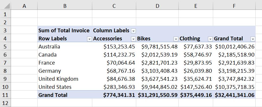
This had to be done with no VBA, no megaformulae, and not in Power BI, but in Excel.
The Solution
You may have thought, hey, applying filters will be easy. I’ll just highlight the columns in the PivotTable that I wish to apply the filters to, navigate to the Data tab on the Ribbon and click on the Filter option in the ‘Sort & Filter’ group.
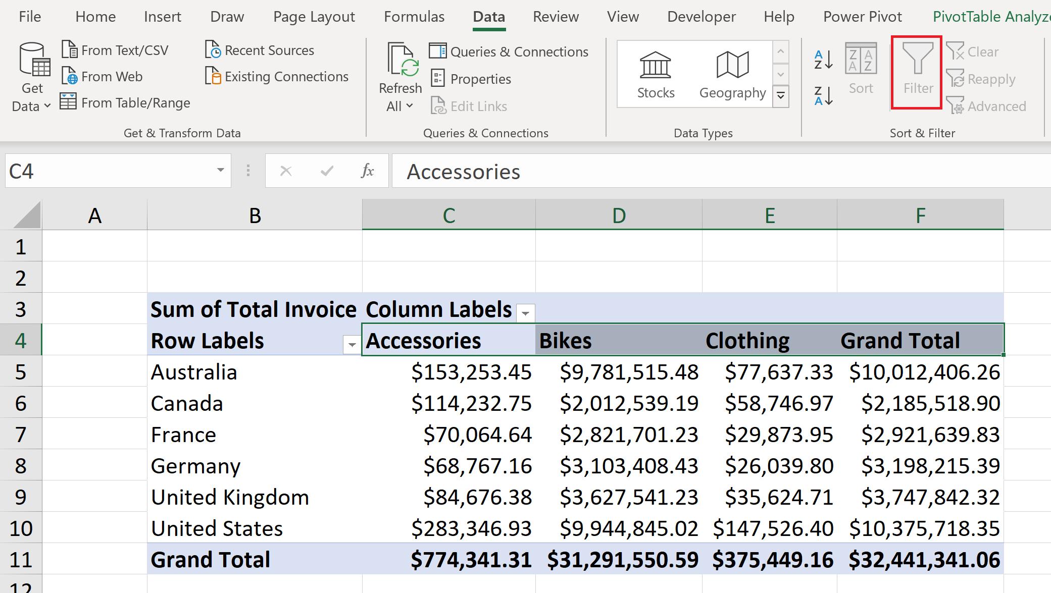
But to your dismay, it is greyed out! So how on earth do we filter the PivotTable? If you thought the challenge was complicated, sit back, grab some scotch, or wine and get ready, this may be a long one. Or perhaps I am practicing poetic licence as this article is really short…
To enable filters on the PivotTable, we click the cell that is located one cell to the right of the top right-hand corner of the PivotTable:
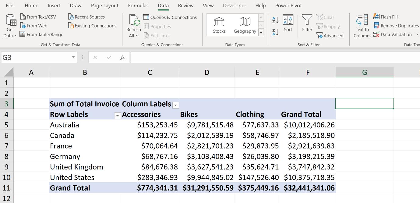
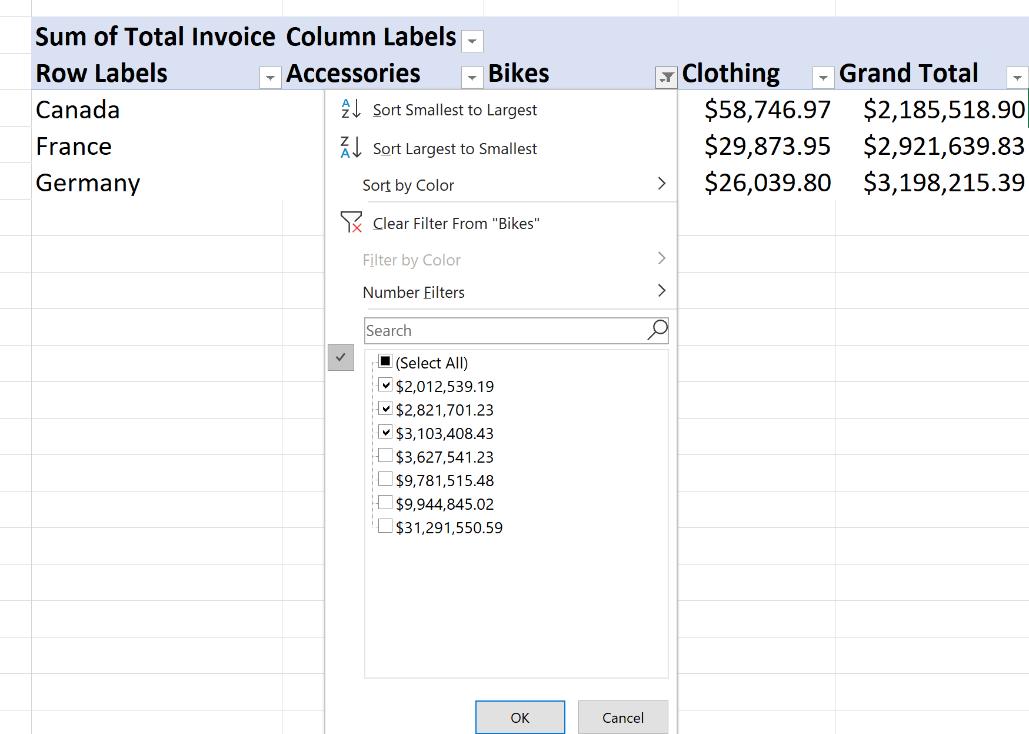
Notice that the Filter option can be now be toggled ‘on’? In fact, this will work for any adjacent cell in column G. We click it and that’s how we get our filters on each column in the PivotTable:
That was a tough one. Hopefully, you have not finished that bottle of alcohol yet! If you have, I suggest professional help – or else invite us round.
The Final Friday Fix will return on Friday 31 July with a new Excel Challenge. In the meantime, please look out for the Daily Excel Tip on our home page and watch out for a new blog every business workday.