Excel for Mac: Filtering by Values in a PivotTable

This week in our series about Microsoft Excel for Mac, we focus on filtering by values in a PivotTable, and how it’s a little different to Windows.

PivotTable filtering on Mac has the same capability as on Windows, but it can be a bit confusing if you have several fields as values and you want to use any other than the first value field in your filter.

Filter the First Value Field – Easy

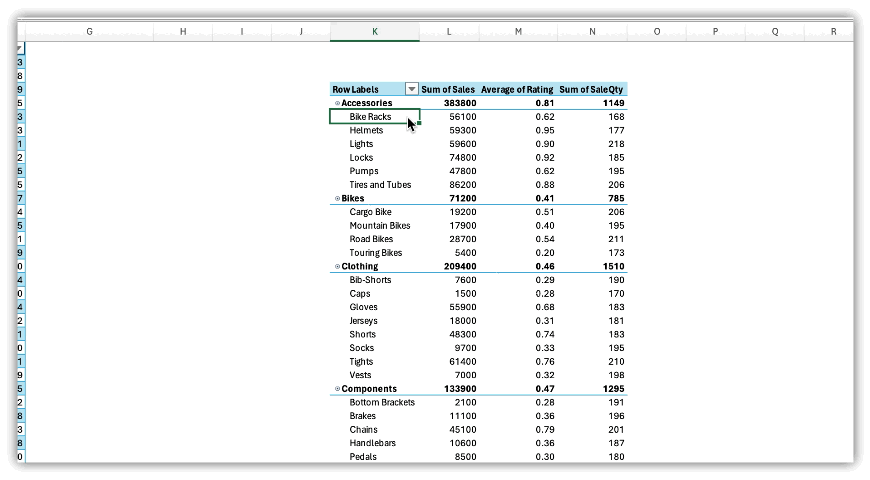
Suppose you have a PivotTable with three [3] value fields, Sum of Sales, Average of Rating and Sum of SaleQty.  If you want to filter for Sum of Sales values greater than a certain amount, it’s very straightforward:

•  Open the Filter dialog for the PivotTable pressing the button in the header
• Press the ‘By value’ pop-up button, and choose the type of filter, such as ‘Greater Than’
• Enter the value for your criteria.

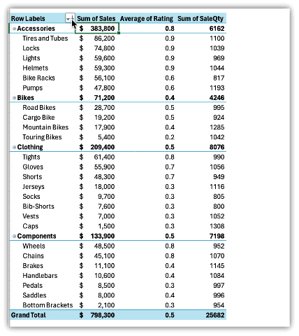
In our example below, we filter for only values greater than 190.  Since the first value field in our PivotTable is Sum of Sales, the filter affects that field.  That’s easy enough to understand, but what if we want to filter on the second or third value field in our table?

If you undertake the steps above on Windows, it will open a dialog where you can pick any of the value fields.  On Mac, finding and opening that dialog is a little different.

Filter on Any Value Field – Not as Obvious

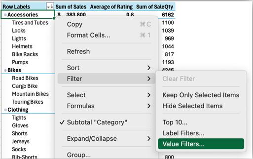
To filter on one of the other value fields, it’s not so straightforward, but it’s still easy if you know where to start.  Instead of pressing the filter button in the row header, you need to open the context menu for one of the row headers.

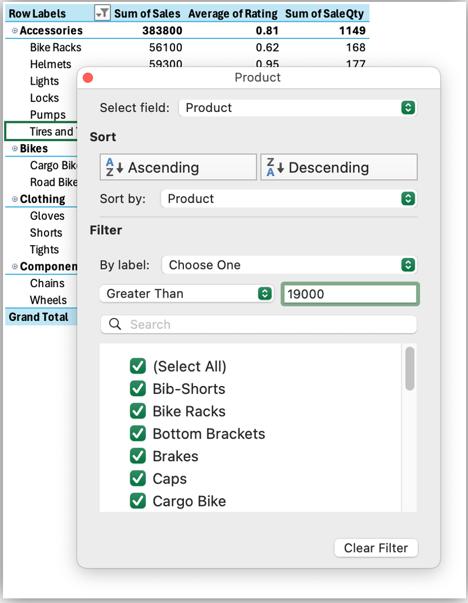
• Select a row headers cell to filter that field by one of the values fields.  In our example, we have Category and Product as our row headers.  To filter the Category, we select a cell that shows one of our categories
• Open the context menu.  There are three [3] ways to do that:

1. SHIFT + Click (hold the SHIFT key and click the cell)
2. Press SHIFT + F10 on your keyboard
3. Right-click the cell (if you have a mouse with a right-click button or if you’ve set your Trackpad to use a secondary click)

• Choose Filter -> Value Filters… as shown in the screen shot below:

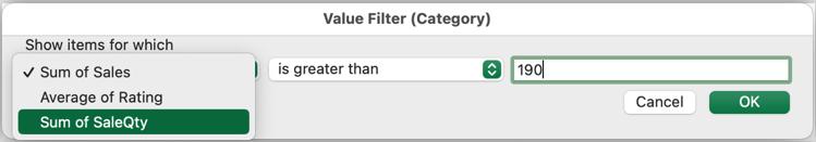
• The ‘Value Filter’ dialog will open.  Notice in our example that Category appears in the title of the dialog, indicating that our filter will apply to the Category field
• Pick which value field you want to filter on, and then set the filter as desired.  For example, in the screen shot below, we select the Sum of SaleQty, choose “is greater than” and type 190
• Press OK to apply the filter.

Below, we have a short video that shows all the steps:

Now you know how to filter on any value field in your PivotTable on a Mac.  Hopefully this was not a problem for you, but if it was, it shouldn’t be any longer.

We hope you find this topic helpful.  Check back for more details about Excel for Mac and how it’s different to Excel for Windows.