Excel at Monopoly #2: MMULT sneak peek

Moving around the board

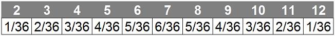
Let’s start off by thinking about probabilities. Every time you play a turn, you roll two six-sided dice, add them together, and move that many squares. These follow a triangle-like distribution with low likelihoods for values closer to 2 and 12, and the highest likelihood for values around 7.

So if we think about the very start of a game of Monopoly, we would start at Go, and have the above probabilities of moving to different squares.

Now, picture what the likelihood of landing on different squares are, over two turns. This is effectively calculated by taking the probability of landing on squares 2-12 from Go, and then multiplying it by the probability of moving from those squares to the next squares.

This is, of course, a slightly simplistic way of looking at it. Although you have a 6/36 chance of landing on Chance (square 7) on the first turn, almost all of the possible cards you might draw will move you to a different location – advance to the nearest railroad, go back three spaces, go directly to Jail, etc..

Probability matrix

Imagine how we can represent this in Excel. We can have a row that asks: for any given starting square, what is the probability of getting to any other square? If we compile all possible starting squares into a table, we get what we refer to as a probability matrix. This reflects the possible outcomes of making a single move, and their relative probabilities.

One of the tricks you can do with a probability matrix is that you can simulate taking multiple moves by multiplying the probability matrix by itself. This is a more advanced form of what we did earlier – instead of looking just at the subset of squares that you can get to from Go, we’re looking at all the possible squares on the board.

Let’s look at a simpler example with only three squares: A, B and C. In this example, if you’re currently on square A, you have a 50/50 chance of ending up in square B and in square C at the end of your turn. If you’re in square B, you have a 25% chance of ending up in square A or square C, but you also have a 50% chance of staying in square B.

Now, if we were to take two steps from square B, what’s the likelihood that we end up back in B?  Well, there are several possibilities: 

• We could go from B to A in our first step (25%), then we could move back to B in the second step (50%).  These steps are reflected by multiplying the yellow squares together
• We could stay in B in our first step (50%), and then also stay in B for our second step too (50%).  This is effectively the same as multiplying the orange square by itself
• We could move to C in our first step (25%) and then move back to B in the second step (40%).  This can be worked out by multiplying the blue squares together.

The total end probability is A (12.5%) + B (25%) + C (10%) = 47.5% (rounded to 48% in the green square above).  So effectively, to get the table on the right, you choose your row in the first table, you choose your column, and then multiply the first items in the row and column by each other, then the second items in the row and column, and so on, then add up the results.

Sounds like a job for SUMPRODUCT, right?  Not quite!

MMULT – matrix multiplication

For those of you who are following the A to Z of Excel Functions series, you may want to cover your eyes to avoid spoilers.  Or, you may want to read on to avoid waiting two years to hear about this nifty function.

SUMPRODUCT will only work when your vectors are moving in the same direction.  What we want to do here is multiply the entire 3x3 matrix by itself to get another 3x3 matrix.  In mathematics, they refer to this as matrix multiplication.  In Excel, we have just the tool for the job – MMULT.  To use it in this context, select a 3x3 range of cells, use the formula =MMULT(<probability matrix>,<probability matrix) and hit Ctrl+Shift+Enter – it has to be used as an array function to populate all the cells, otherwise Excel will only calculate the top left corner.

Steady state

The final step (pardon the pun) is to see what happens if you just keep going round and round the board.  If you keep multiplying the probability matrix by itself, the probabilities end up converging to what is referred to as a steady state.  At this stage, it doesn’t matter if you take 100 steps or 10,000 steps, you’re pretty much just as likely to end up on the same squares either way.

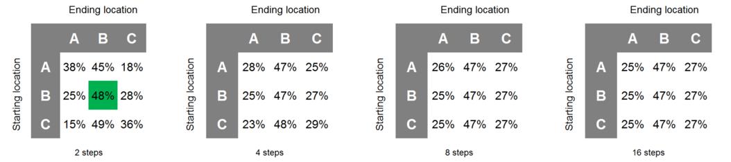
What you may also notice is that the probabilities on each line start to align as well. What this tell us is that after 16 steps in our little 3x3 board, it doesn’t matter where you start off, you’re just as likely to end up in any given square. These final probabilities can effectively be thought of as the long-term likelihood of anybody landing on any of these squares.

Now, if we extend the scale of what we’re doing back to the Monopoly board, we end up with the following probabilities that we saw in last week’s blog:

If we think about these further, we can consider why they come about:

• It’s impossible to end your turn on ‘Go to Jail’
• If you’re stuck in jail, you can spend up to three turns there
• Chance cards frequently transport you to other squares
• The higher probability ‘normal’ squares are 1-2 die rolls away from Jail, the most probable square
• The lower probability ‘normal’ squares are 1-2 die rolls away from Go to Jail, the least probable square.

Next week, we’ll look at turning this data into valuable information you can use to make better decisions in your games. See you next week!