Challenges: Monday Morning Mulling: October 2018 Challenge

On the final Friday of each month, we set an Excel problem for you to puzzle over for the weekend. On the Monday, we publish a solution – or two as in this case. If you think there is an alternative answer, feel free to email us. We’ll feel free to ignore you.

Final Friday Fix: October Challenge Recap

As explained on Friday, a positive integer (whole number) is said to be prime if and only if two different integers divide it: one (1) and itself. Therefore, 1 is not prime and 2 is the only even prime etc.

The challenge this month was extremely straightforward:

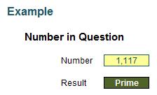
All you had to do was write a formula in Excel to determine whether a number typed in (as above) is prime or not.  That was it – just no VBA (or JavaScript!) / user defined functions. 

Suggested Solution(s)

This month’s query then is, how do I determine if a number is prime?  You might think, I couldn’t care less.  But please keep reading.  This month’s article is not so much about getting the right formula but more about, er, getting the formula right in general.

THE INTERNET LIES TO YOU.

That’s right.  Before you switch off, this month’s question raises a very important point that affects us all.  Let me explain.  I want to determine whether a number in a particular cell, let’s call it Number, is prime or not, e.g. (as above)

Let’s do something different this month.  I am going to search for a solution to this problem on the internet.  I know, who would have thought?  I bet you’ve never done it.  It doesn’t take too much effort to locate one of two very popular solutions, either

or

They have four things in common:

1. They are both array functions (i.e. entered using CTRL + SHIFT + ENTER – you do not try and type the braces ({ and }) in
2. These solutions are cited all over the internet, including on esteemed websites like Microsoft’s own Excel Blog
3. They are both fairly incomprehensible upon initial inspection
4. Neither actually work.

Yup, read point 4 again.  They’re wrong.  They don’t work in all situations – and yet they seem to be universally accepted.  And that’s the point of today’s blog.  When we don’t know how to do something, you head for your favourite search engine, hunt out the answer – and if you are wiser, check four or five sites to ensure they come to the same conclusion before accepting that answer. 

These formulae would pass that sniff test.  That’s my point.  But they are still wrong.

To show they don’t work, simply download this month’s attached Excel file, then try these:

• Apparently, 1.7 is prime
• With the first formula, the value 0 (zero) gives #REF!
• With the second formula, the value 1 gives #REF!
• Negative numbers give #NUM!

Nobody tests anything anymore.  We are all download drones.  And this scares the living daylights out of me.  People might try numbers like 2, 17, 59, etc. and see it seems to work and conclude everything is fine.  But just because something is on page 1 of a well-known search engine page doesn’t make it true.  If you don’t believe me, Google it.

For the record, I made an attempt in the past – which worked for a while, and then OFFSET changed its behaviour!  So please find below my latest and greatest attempt at a solution:

That’s right – it’s even worse than the other two.  In the next section, I’ll explain how this formula works, but feel free to stop reading at this juncture.  Showing off some horrendous calculation is not the objective of this article.  It’s realising that you have to be careful when reading articles on how to solve things in Excel.  Yes, that includes my articles too (because – as I said above – my original solution no longer works).

How the Formula Works

You don’t have to read this!  If you are interested though, the formula

needs to be picked apart. However, before I do that, I need to show you a quick way to check for a prime. Consider the divisors of 60:

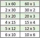
Do you see the symmetry?  Once you get to the middle – the square root – the factorisation reverses.  Since the square root of 60 is slightly less than 8, I only need to test to see if the numbers 1 to 8 divide 60.  Given 1 and n will always divide n, I really only need to test the numbers 2 to ROUNDUP(SQRT(n),0) (the square root of n rounded up to the next whole number), which is 8 here.  This saves a lot of needless calculations!

This explains the element highlighted:

The function OFFSET(Reference, Rows, Columns, [Height], [Width]) has been discussed previously (see the article Onset of Offset for further details). 

The formula OFFSET($A$2,,,ROUNDUP(SQRT(Number),0)-1) gives a range of A2 to A8 if Number were 60 (1 has to be subtracted otherwise with a height of 8, you would get the range A2:A9).  Putting ROW() around this expression is a crafty way to convert to the numbers 2 to 8 inclusive.  This is why cell A2 must be a cell reference on row 2 in this example.

The next key element is MOD(Number, Divisor).  Again, I have discussed MOD before (please see A Modicum of MOD for further details): this provides the remainder after dividing Number by Divisor.  So, if I divide Number by each Divisor for the numbers 2 to ROUNDUP(SQRT(Number),0) – which would be 2 to 8 if Number were 60 – and any division gives me zero, that would mean Number is divisible by Divisor, i.e. the number is not prime.  If no division gives zero, it has to be prime so

gives the appropriate prime / not prime identification in certain circumstances.  This formula is both a variation of my proposed one and the second one identified as wrong earlier.  Do note it is encapsulated in an AND function and is in an array formula.  This forces Excel to perform all of the calculations from 2 to ROUNDUP(SQRT(Number),0) in one cell.  That’s a useful way of using an array formula (for more on arrays, please see Array of Light).

The rest of my formula,

is made up of tweaks to ensure:

• Non-integers are not prime
• 0 is neither prime nor an error
• 1 is neither prime nor an error
• Negative numbers are neither prime nor an error.

My formula goes wrong eventually.  9 x 10²⁰⁰ is clearly not prime (it’s 3 x 10¹⁰⁰ squared) but Excel cannot evaluate it because it’s too large.  Meh, you can’t have everything!

Incidentally in the attached Excel file, as well as showing the oft-quoted – but wrong – solutions and my revised attempt above, I have added an alternative solution:

This solution uses the brand new to Office 365 Dynamic Arrays, using the SEQUENCE function to convert the consecutive numbers.  Note it doesn’t require an array (CTRL + SHIFT + ENTER) formula.  Please note for most people this formula will give rise to an error, as these functions and features are not yet Generally Available in Excel – but it’s worth noting for the future.

If it does work, my first solution will be revised using SINGLE and no longer require braces (‘{‘ and ‘}’):

Word to the Wise

Keep reading these articles but stay cynical. I am as prone to mistakes as the next persona (that’s a joke!). By all means research, but convince yourself that it’s right. Take nothing at face value.

The Final Friday Fix will return on Friday 30 November with a new Excel Challenge. In the meantime, please look out for the Daily Excel Tip on our home page and watch out for a new blog every business workday.