Challenges: Monday Morning Mulling: February 2019 Challenge

On the final Friday of each month, we set an Excel problem for you to puzzle over for the weekend.  On the Monday, we publish a solution.  If you think there is an alternative answer, feel free to email us.  We’ll feel free to ignore you.

Welcome to this month’s Monday Morning Mulling.  Can you work around the foibles of data validation?

Last week, we posed an interesting problem – data validation warnings can help you check a value you enter into a cell, ensuring that it either comes from a pre-defined list, or to confirm that you want to add your value to the cell.  The problem arises in this specific scenario, where a new value will add to the list in a dynamic way, because a formula-driven list will pick up the value before the data validation check is applied.  Because of this, when the data validation is checked, it sees the value in the list, and proceeds to treat it as a valid value.

So, how do we get around this?

First of all, we need to create a dynamic list using range names.  Rather than go into a big explanation of how that works, I’m going to leave this convenient article on Dynamic Range Names that we’ve written for precisely this reason.  In particular, we’re going to use the OFFSET approach, but it doesn’t matter too much.

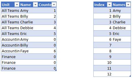
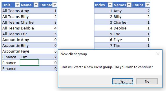
I’m firstly going to create a counter to keep track of which names already exist in my list.  This will form the basis of my named range.  We can use the formula:

The idea is that we’re going to look through the Name column and check to see if this is the first instance of the name appearing.  If so, we’re going to increment a counter.  So if this is a value contains the fifth unique name in the list, it will have a counter result of ‘5’.

Off somewhere else in the spreadsheet, we can create an index that looks at the numbers we have assigned, and form them into a list.  This is simply an INDEX(MATCH) function to pull things into line, such as:

The MATCH function finds the first instance of the name, and the INDEX function pulls it into a table so that we can put it into our named range accordingly.

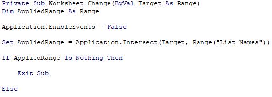
So far, so good.  Now, here’s where it’s tricky.  Adding a new name updates the list of names faster than the data validation can check for, so it won’t warn us when we’re putting a new name in.  To get around this and provide the warning that we’re looking for, we’re going to need a macro to help us out.

The macro is going to run every time we make a change to the worksheet, to test if we actually want to keep or reject the value that we’ve just entered.  We’ll check whether the change exists in the area that we’re targeting, and if not, then we’ll ignore the rest of the macro.  We can do this with the following code (assuming that your data validated cells are in the range called “List_Names”:

Once we have identified that we’re working in the data validated cells, we need to check off a few things that will invalidate our results.  If we’re selecting multiple cells, that will cause us issues, so we need to set up an error trap if that’s the case.  Also, if we’re deleting a value, rather than adding a new name in place, we don’t want to run the code either – no need to data validate our deletion.  So we need the following items as well:

Ok, now we’re at the stage where we need to test if our names have appeared before. We can call a MATCH function to check where the name appears in our list, and an INDEX(MATCH) to determine how many times it’s appeared thus far.

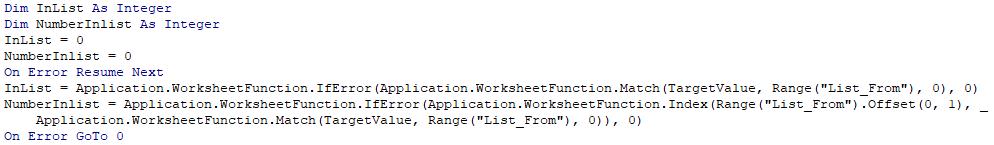
So here’s the sneaky bit now.  If the name we’ve just entered appears exactly once, then we know that it didn’t exist previously in the list.  So, we can test to see if the number of times it’s appears is greater than 1.  If so, then we don’t need to do run any warning, because the data validation is working the way we want it to.

However, if there is exactly one item in the list, then we want to pop up a message box and check to see if we really do want to enter it and add it to the list.  If not, we should delete the value that was just entered.  That’s what this next block of code does:

A MsgBox function will return a value based on what button is clicked. In our case, clicking the “Yes” button when it asks you if you want to continue gives us a value of ‘6’, which we can check for. If the value returned doesn’t equal 6 (e.g. if the user clicks on no, cancel, or anything else), then the cell we’re looking at will have the contents removed, and it will effectively undo the act of typing a new name in place.

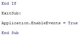
Finally, just the clean-up at the end to reenable events (we disabled it initially because deleting the value would also trigger this check!) and to provide a break place (here called ExitSub) to allow errors to skip through the main code content.

All this is here to give us the popup result that we’re looking for:

How did you go?  Did you find a formula-based solution that didn’t require VBA?  Let us know, we’d be keen to hear if you think you have a better way to do this!  You can find an example of our solution here. Otherwise we’ll see you next month for our next Final Friday Fix!

The Final Friday Fix will return on Friday 29 March with a new Excel Challenge.  In the meantime, please look out for the Daily Excel Tip on our home page and watch out for a new blog every business workday.