
Challenges: Monday Morning Mulling: April 2021 Challenge
3 May 2021
On the final Friday of each month, we set an Excel / Power Pivot / Power Query / Power BI problem for you to puzzle over for the weekend. On the Monday, we publish a solution. If you think there is an alternative answer, feel free to email us. We’ll feel free to ignore you.
This month, we want to check if a pair of values are of the same category.
The Challenge
To identify commonality in different values and distinct categories can sometimes be difficult. For instance, I came across a dataset that shows which social media channels certain SumProduct staff members use:

Imagine that this data set goes on to for 1,000 rows. Using this data set as an example, how hard it is to identify if a pair of users have a common social media channel?
The challenge was “simply” this: could you write a formula to potentially create a list of pairs that use a common social media channel. This must be done in one cell. We even supplied a starter file for you!
Suggested Solution
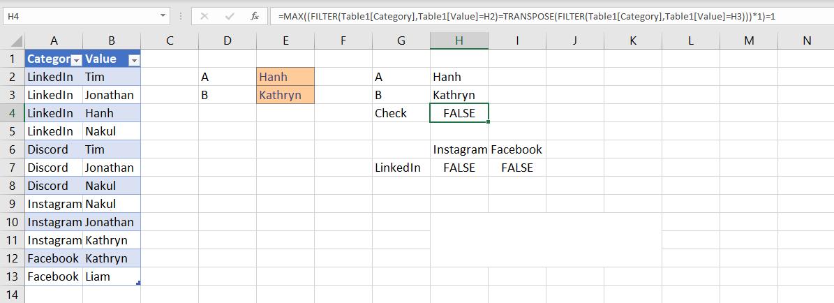
To start off with, we need to identify what platforms each staff member uses. We will create two lists of social media channel that are to be used to compare both users. I will first start with the ‘User A’ (Hanh). Using the FILTER dynamic array function, I will create a dynamic array in G7 using the following formula
=FILTER(Table1[Category],Table1[Value]=H2)
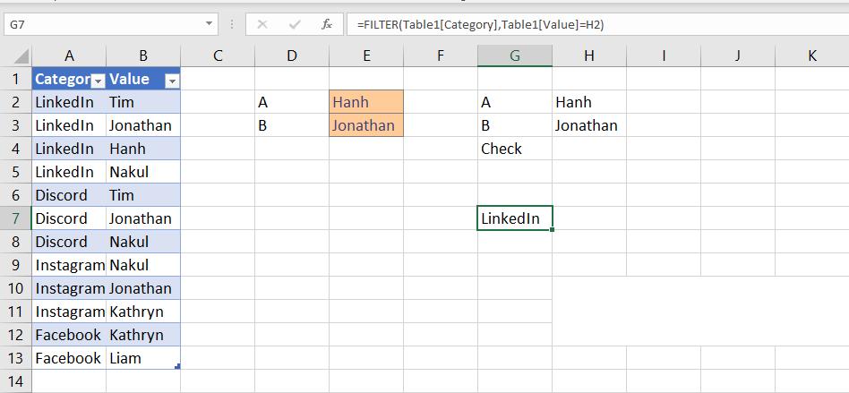
As expected, the only platform ‘User A’ uses is LinkedIn. Now moving to ‘User B’ (Jonathan), I transpose the list of social media channels to create an array in H6 using
=TRANSPOSE(FILTER(Table1[Category],Table1[Value]=H3))
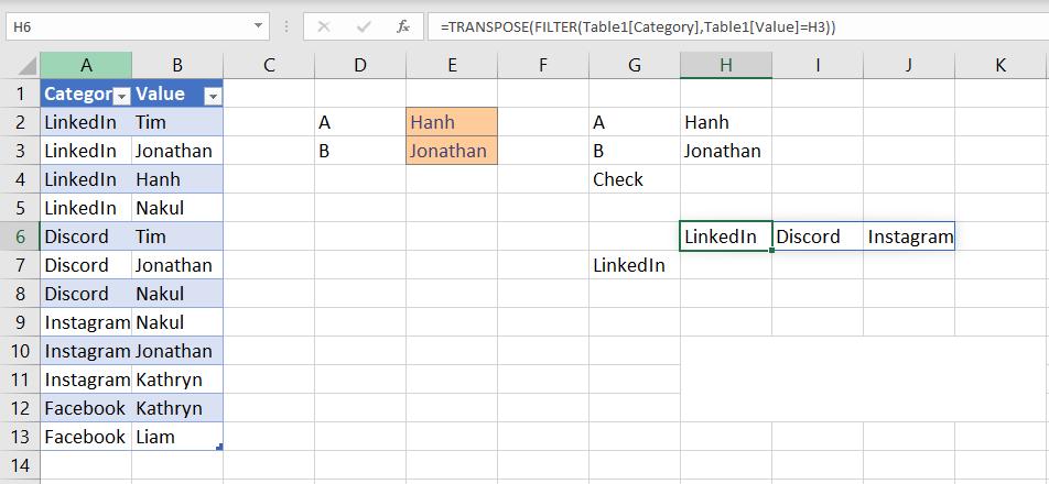
From the data, ‘User B’ uses LinkedIn, Discord, and Instagram.
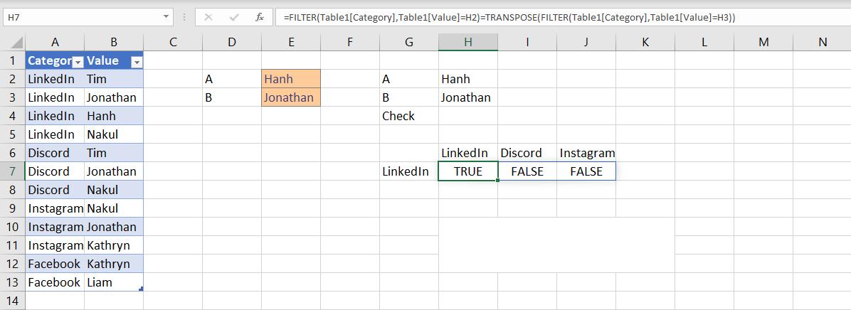
Now the question is, how do we pair up the list? The answer is simple: we just check if list A equals list B in H7 by using the following formula
=FILTER(Table1[Category],Table1[Value]=H2)=TRANSPOSE(FILTER(Table1[Category],Table1[Value]=H3))
Now we finally check if the users share a social media channel in H4 using
=MAX((FILTER(Table1[Category],Table1[Value]=H2)=TRANSPOSE(FILTER(Table1[Category],Table1[Value]=H3)))*1)=1
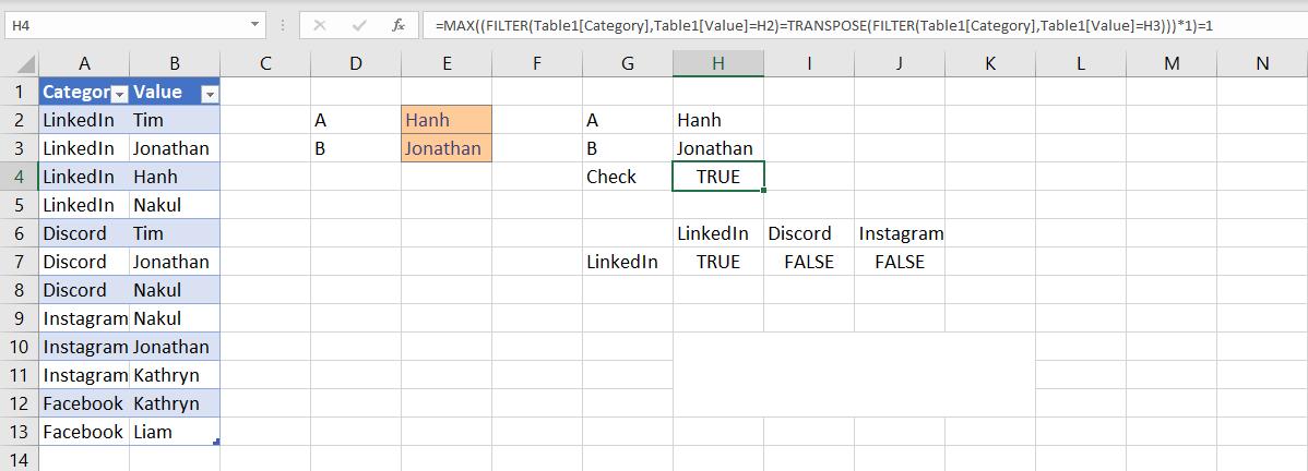
There it is! For my satisfaction I will try a different user by changing cell E3 and I get the following
Thankfully, it works! You have a check that displays if a pair of users are active on a social media cannel. This file contains the worked solution.
Until next month!
The Final Friday Fix will return on Friday 28 May 2021 with a new Excel Challenge. In the meantime, please look out for the Daily Excel Tip on our home page and watch out for a new blog every business workday.