A to Z of Excel Functions: The SINGLE function

Welcome back to our regular A to Z of Excel Functions blog.  Today we look at the SINGLE function.

The SINGLE function

SINGLE was one of seven functions heralding the new dawn of arrays – the Dynamic Array.

Before explaining SINGLE, let’s first consider what a Dynamic Array is.  Consider the following data:

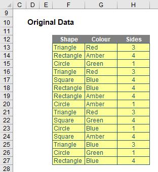
If I were to type =F12:H27 into another cell, Excel in the past would have thought I had gone mad.  I’d need to wrap it in an aggregation function such as SUM, COUNT or MAX, to name but a few.  Otherwise, I would have to wrap it in braces using CTRL + SHIFT + ENTER and use it as an array formula.

But no more.

Look at what happens when I type =F12:H27 into cell F33:

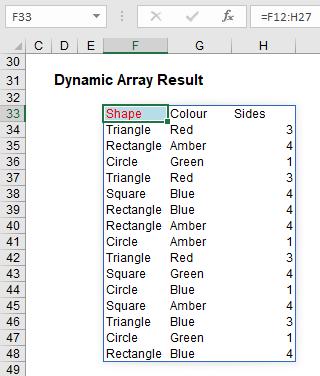
The formula automatically extends to three columns by 16 rows!  It has spilled.

Any formula that has the potential to return multiple results can be referred to as a Dynamic Array formula.  Formulae that are currently returning multiple results, and are successfully spilling, can be referred to as Spilled Array Formulae.

Notice I did not have to highlight all of the cells F33:H48.  It spilled.  Also take note I formatted cell F33 – er, that didn’t spill, because formatting doesn’t propagate.

And don’t let this basic example put you off either.  If you feel a general sense of underwhelm coming over you, it’s because I haven’t yet communicated how powerful this all is as my example was too basic.

However, before I carry on there is a question I do need to cover with my far too simple example: what happens if something gets in the way?

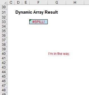
In this example, in cell G40, I have typed in the obtrusive text, “I’m in the way”.  And it quite literally is.  Consequently, I have generated the #SPILL! error.  The formula cannot spill, so the error message is generated accordingly. 

#SPILL! Errors

#SPILL! errors are returned when a formula returns multiple results, and Excel cannot return the results to the spreadsheet.  There are various reasons an #SPILL! error could occur:

• spill range is not blank: as in my example (above), this error occurs when one or more cells in the designated spill range are not blank and thus may not be populated. 

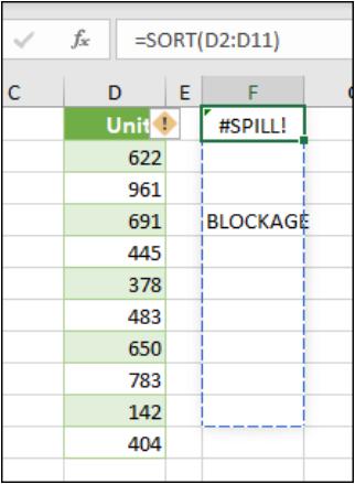
When the formula is selected, a dashed border will indicate the intended spill range.  You may select the error “floatie” (believe it or not, this is what Microsoft call these things!), and choose the ‘Select Obstructing Cell’ option to immediately go the obstructing cell.  You can then clear the error by either deleting or moving the obstructing cell's entry.  As soon as the obstruction is cleared, the array formula will spill as intended

• the range is volatile in size: this means the size is not “set” and can vary.  Excel was unable to determine the size of the spilled array because it's volatile and resizes between calculation passes.  For example, the new function SEQUENCE(x) generates a list of x numbers increasing by 1 from 1 to x.  That’s fine, but the following formula will trigger this #SPILL! error:

Dynamic array resizes may trigger additional calculation passes to ensure the spreadsheet is fully calculated.  If the size of the array continues to change during these additional passes and does not stabilise, Excel will resolve the dynamic array as #SPILL!  This error type is generally associated with the use of RAND, RANDARRAY and RANDBETWEEN functions.  Other volatile functions such as OFFSET, INDIRECT and TODAY do not return different values on every calculation pass so tend not to generate this error

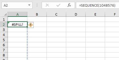
• extends beyond the worksheet’s edge: in this situation, the spilled array formula you are attempting to enter will extend beyond the worksheet's range.  You should try again with a smaller range or array.  For example, moving the following formula to cell A1 will resolve the error, and the formula will spill correctly

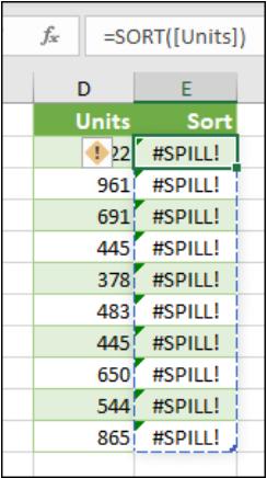
• Table formula: Tables and Dynamic Arrays are not yet best friends.  Spilled array formulae aren't supported in Excel Tables (generated by CTRL + T).  Try moving your formula out of the Table, or go to Table Tools -> Convert to range

• out of memory: I have forgotten what this one means.  Sorry, I couldn’t resist that.  The spilled array formula you are attempting to enter has caused Excel to run out of memory.  You should try referencing a smaller array or range
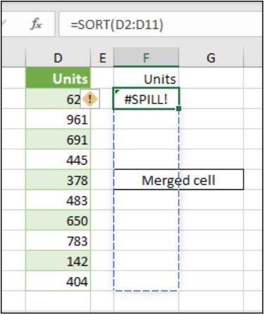
• spill into merged cells: spilled array formulae cannot spill into merged cells.  You will need to un-merge the cells in question or else move the formula to another range that doesn't intersect with merged cells.

When the formula is selected, a dashed border will indicate the intended spill range.  You can again select that wonderfully named error floatie and choose the ‘Select Obstructing Cell’ option to immediately go the obstructing cell.  As soon as the merged cells are cleared, the array formula will spill as intended

• unrecognised / fallback error: the “catch all” variant.  Excel doesn't recognise, or cannot reconcile, the cause of this error.  Here, you should make sure your formula contains all of the required arguments for your scenario.

Returning to Dynamic Arrays

Now that we have considered what happens if you block a Dynamic Array, let me now turn my attention to what happens if you don’t.  You get the following:

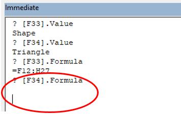
Do you see I am not having to anchor cells (i.e. use dollar [$] signs)?  The formula just spills.  Let me be clear.  If I select cell F34, I get the following:

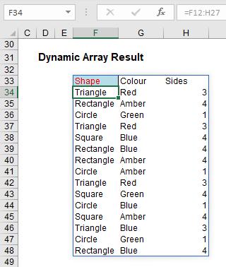
Here’s a first.  Check out the formula in the formula bar.  It’sgreyed out.  Ever seen that before?  Effectively, cell F34 contains the value ‘Triangle’ but it does not actually contain an “Excel” formula in the usual sense.  To demonstrate this, let me show you the VBA Immediate Window:

If you select cells F33:H48 and use ‘Go To Special’ (F5 -> Special), and then select ‘Formulas’, cells F33:H48 are shown as formula cells.  You can even copy and paste them as values.  Ladies and gentlemen, welcome to this brave new world.

Once you have a Dynamic Array, referring to it is simple using what is known as the Spilled Range Operator.  For example, if I want to refer to the Dynamic Array in the previous examples, it initially had a range of L57:N72.  However, once I had added a row and column to the Table, this resized to L57:O73.  I can easily refer to this array, whatever its size as follows.  In its initial state:

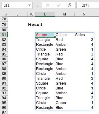
The formula =L57# allows for variations – you simply type in the top left-hand cell reference (i.e. the cell with the non-greyed out formula) and add ‘#”, known as the Spilled Range Operator.  Simple!

Implicit Intersection Implications

It may be an alliteration and sound like something you can get arrested for, but Dynamic Arrays do come at a price.  There aren’t many users out there who used them, but there are some – and hence there will be some legacy calculations affected. 

In the past, if you entered =A$1:A$10 anywhere in rows 1 through 10, the formula would return only the value from that row.  In fact, a spreadsheet our company is presently auditing relies on this behaviour.  However, in the brave new world of Office 365 (albeit selected Insider recipients for the time being), typing this formula would create a Spilled Array Formula.  To protect existing formulae, we need a new – if not instantly breathtaking – function…

SINGLE Function

With the above discussion borne in mind, SINGLE is essential to keep Excel running smoothly, but it’s probably safe to say it won’t set the world alight.  The SINGLE function returns a single value using logic known as implicit intersection.  SINGLE may return a value, single cell range or an error.

The function has the following syntax:

The function has just one argument:

• value: this argument is required and represents the array to be selected.

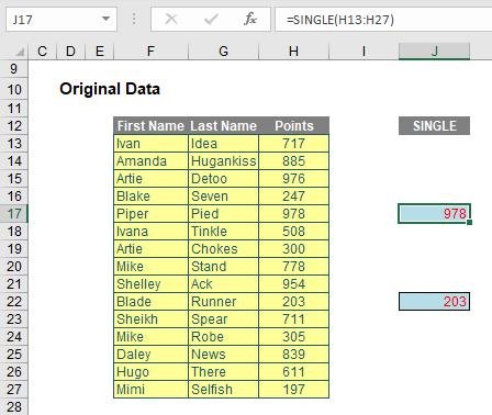
When the supplied argument is a range, SINGLE will return the cell at the intersection of the row or column of the formula cell.  Where there is no intersection, or more than one cell falls in the intersection, then SINGLE will return a #VALUE! error.  When the supplied argument is an array, SINGLE returns the first item (Row 1, Column 1).

In the example below, the two SINGLE formulae are supplied a range, H13:H27, and return the values in cells H17 and H22 respectively.

I can see an argument going forward that some form of OFFSET (e.g. “NEXT” or “PRIOR”) may be needed in due course – but no one is expecting everything to come together on Day 1.

Dynamic Arrays vs. Legacy Array Formulae

Prior to this new functionality, if you wanted to work with ranges in Excel, you used to have to build array formulae, where references would refer to ranges and be entered as CTRL + SHIFT + ENTER formulae.  The main differences are as follows:

• Dynamic Array formulae may spill outside the cell bounds where the formula is entered.  The Dynamic Array formula technically only exists in the cell in the top left-hand corner of the spilled range (as shown earlier), whereas with a legacy CTRL + SHIFT + ENTER formula, the formula would need to be entered in the entire range
• Dynamic arrays will automatically resize as data is added or removed from the source range. CTRL + SHIFT + ENTER array formulae will truncate the return area if it's too small, or return #N/A errors if too large
• Dynamic array formulae will calculate in a 1 x 1 context
• Any new formulae that return more than one result will automatically spill.  There's simply no need to press CTRL + SHIFT + ENTER
• According to Microsoft, CTRL + SHIFT + ENTER array formulae are only retained for backwards compatibility reasons.  Going forward, you should use Dynamic Array formulae instead
• Dynamic array formulae may be easily modified by changing the source cell, whereas CTRL + SHIFT + ENTER array formulae require that the entire range be edited simultaneously
• Column and row insertion / deletion is prohibited in an active CTRL + SHIFT + ENTER array formula range.  You first need to delete any existing array formulas that are in the way.

We’ll continue our A to Z of Excel Functions soon.  Keep checking back – there’s a new blog post every business day.

A full page of the function articles can be found here.