
A to Z of Excel Functions: The MUNIT Function
19 September 2022
Welcome back to our regular A to Z of Excel Functions blog. Today we look at the MUNIT function.
The MUNIT function

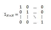
In matrix algebra, the MUNIT function returns the unit matrix for the specified dimension. A unit matrix is simply a square (n x n) matrix which has the value of one [1] down the leading diagonal (from top left to bottom right) and zero [0] everywhere else.
Described like this, it doesn’t sound very exciting!
It has the following syntax:
MUNIT(dimension)
The MUNIT function has the following argument:
- dimension: this is required and represents an integer specifying the dimension of the unit matrix that you wish to return, resulting in a square (n x n) array. This dimension must be greater than zero [0].
It uses the following equation:
If dimension is a value less than or equal to zero [0], MUNIT returns the #VALUE! error value.
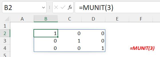
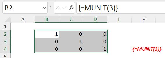
If you are using Microsoft 365, then you can simply enter the formula in the top left-cell of the output range and then press ENTER to confirm the formula as a dynamic array formula. Otherwise, the formula must be entered as a legacy array formula by first selecting the output range, entering the formula in the top-left-cell of the output range, and then pressing CTRL + SHIFT + ENTER to confirm it. Excel inserts curly brackets (known as braces) at the beginning and end of the formula for you.
In Excel 365:
In a “legacy” version of Excel:
So what would you use this function for?
Let’s keep this simple, and just consider a 2 x 2 matrix scenario. Matrices are used to transform data, often used in computer graphics, cartoons, etc. Sometimes, you wish to maintain a character’s direction or bringing it nearer or closer (scaling up or scaling down).
In linear algebra, the term eigenvector is used to denote the direction that should remain consistent. The corresponding term eigenvalue would denote the scale of the enlargement, e.g.
- 1 would mean “no change”
- 2 would mean “double the length”
- -1 would mean point in the opposite direction to the eigenvalue.
Of course, mathematicians (such as myself!) have to complicate this notion in case someone still understands what I am talking about. It may be represented mathematically in the form
Av = λv
where:
- A is a matrix of dimension n x n
- v is a vector, consisting of one row or one column, with n elements. This is the eigenvector
- λ is the scalar multiple (i.e. it is simply a number) which represents the eigenvalue.
[For what it’s worth, “eigen” comes from the German word for “typical”, if that helps clarify.]
As an example, let’s consider the 2 x 2 matrix

This has an eigenvector of with an associated eigenvalue of five [5].
How on earth was this calculated? Let’s revert to the original premise:
Av = λv
To ensure I am considering like with like, I will make sure both sides of the equation are matrices, so I will add the 2 x 2 identity matrix, i.e. MUNIT(2) here:
Av = λIv
where I is the unitary 2 x 2 matrix. Thus:
Av – λIv = 0
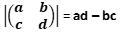
Assuming the eigenvector v is non-zero, we may solve for the eigenvalue λ by calculating the determinant of the matrix. This is a special calculation in linear algebra, denoted by |A|, meaning the determinant of the square matrix A. For a 2 x 2 matrix, the determinant is calculated as
To solve for λ, we calculate
|A – λI| = 0
Therefore,
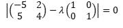
which reduces to
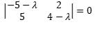
Calculating this determinant, we get
(-5 – λ)(4 – λ) – (2 x 5) = 0
Which simplifies to a quadratic equation, viz.
λ2 + λ – 30 = 0
which is
(λ + 6)( λ – 5) = 0
i.e. λ equals either -6 or +5. That means there are two distinct eigenvalues, one of which is five [5]. Knowing this, we may now calculate the associated eigenvector:
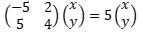
Using standard matrix algebra, we get the two equations
-5x + 2y = 5x
5x + 4y = 5y
Bringing all values over to the left-hand side of the equations, we get
-10x + 2y = 0
5x – y = 0
Clearly, y = 5x, so an eigenvector is any non-zero multiple of the vector. For example,
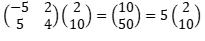
i.e. Av = λv
If you wanted to calculate this in Excel, you would need MUNIT. Further, if you add up the digits on the leading diagonal (known as the trace of the matrix), you will note
-5 + 4 = -1
The two solutions for λ are -6 and +5, which also add up to -1. This is because the sum of the eigenvalues of a matrix equals the trace of that matrix. This can be a good check, which MUNIT may also be used for:
trace(A) =SUM( A * MUNIT(ROWS(A)) )
So ends today’s mathematics lesson. Class dismissed.
We’ll continue our A to Z of Excel Functions soon. Keep checking back – there’s a new blog post every other business day.
A full page of the function articles can be found here.