A to Z of Excel Functions: The IPMT Function

Welcome back to our regular A to Z of Excel Functions blog. Today we look at the IPMT function.

The IPMT function

Imagine I were to borrow $300,000 over 25 years at an interest rate of 6% p.a. Assuming no final amount to pay (i.e. no bullet repayment) and payments were made monthly at the end of each month (“in arrears”), interest would accrue over the month at 6%/12 = 0.50% per month (since there would be no compounding of interest monthly as it would be paid each month and I will simplify that all months are of equal length).

Using Goal Seek, the PMT function or algebraic methods, I could soon determine the monthly payment would be $1,932.90:

You can see that over the 300 months the outstanding balance reduces to zero from an initial loan of $300,000.  The monthly payments (column H) remain constant, but the interest reduces as it calculates the opening balance (for payments in arrears, i.e. the repayment is not included) multiplied by the monthly interest rate, e.g. for cell I29, interest is calculated as

As long as you calculate this table, the formulae are simple.  But what if you don’t want to have to generate this time every time you wanted to know the interest element of the monthly payment for a given month?  You may use the IPMT function, which will give the same solution, but be negative instead.  This is because Excel’s financial functions distinguish between cash inflows (positive) and outflows (negative). 

It employs the following syntax to operate:

The PPMT function has the following arguments:

• rate: this is required and represents the constant interest rate for the loan
• per: this is required, and specified the period to be considered, between periods 1 and nper
• nper: this is also required and denotes the total number of payments for the loan
• pv: also necessary, this is the present value, or the total amount that a series of future payments is worth now, also known as the principal (i.e. what you are borrowing)
• fv: this is the first of two optional arguments.  This is the future value, or a cash balance you want to attain, after the last payment is made.  If fv is omitted, it is assumed to be zero (0), i.e. the future value of a loan is nil
• type: this final argument is also optional.  This the number zero (0) or one (1) and indicates when payments are due:

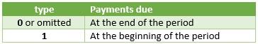
It should be further noted that:

• the interest payment returned by IPMT relates to interest but considers no effect from taxes, reserve payments or other fees sometimes associated with loans
• make sure that you are consistent about the units you use for specifying rate and nper. If you make monthly payments on a four-year loan at an annual interest rate of 12%, use 12%/12 for rate and 4*12 for nper. If you make annual payments on the same loan, use 12% for the rate and 4 for nper.

We’ll continue our A to Z of Excel Functions soon. Keep checking back – there’s a new blog post every other business day.