A to Z of Excel Functions: The INTERCEPT Function

Welcome back to our regular A to Z of Excel Functions blog. Today we look at the INTERCEPT function.

The INTERCEPT function

Sometimes, you wish to forecast what comes next in a sequence, i.e. make a forecast. There are various approaches you could use:

• Naïve method: this really does live up to its billing – you simply use the last number in the sequence, e.g. the continuation of the series 8, 17, 13, 15, 19, 14, … would be 14, 14, 14, 14, … Hmm, great

• Simple average: only a slightly better idea: here, you use the average of the historical series, e.g. for the continuation of the series 8, 17, 13, 15, 19, 14, … would be 14.3, 14.3, 14.3, 14.3, …

• Moving average: now we start to look at smoothing out the trends by taking the average of the last n items. For example, if n were 3, then the sequence continuation of 8, 17, 13, 15, 19, 14, … would be 16, 16.3, 15.4, 15.9, 15.9, …

• Weighted moving average: the criticism of the moving average is that older periods carry as much weighting as more recent periods, which is often not the case. Therefore, a weighted moving average is a moving average where within the sliding window values are given different weights, typically so that more recent points matter more. For example, instead of selecting a window size, it requires a list of weights (which should add up to 1). As an illustration, if we picked four periods and [0.1, 0.2, 0.3, 0.4] as weights, we would be giving 10%, 20%, 30% and 40% to the last 4 points respectively which would add up to 1 (which is what it would need to do to compute the average).

Therefore the continuation of the series 8, 17, 13, 15, 19, 14, … would be 15.6, 15.7, 15.7, 15.5, 15.6, …

All of these approaches are simplistic and have obvious flaws. We are using historical data to attempt to predict the next point. If we go beyond this, we are then using forecast data to predict further forecast data. That doesn’t sound right. We should stick to the next point. Since we are looking at a single point and we can weight the historical data by adding exponents to the calculation, this is sometimes referred to as Exponential Single Smoothing.

A slightly more sophisticated method is called regression analysis: well, that takes me back! This is a technique where you plot an independent variable on the x (horizontal axis) against a dependent variable on the y (vertical) axis. “Independent” means a variable you may select (e.g. “June”, “Product A”) and dependent means the result of that choice or selection.

For example, if you plotted your observable data on a chart, it might look something like this:

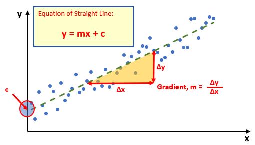
Do you see?  You can draw a straight line through the data points.  There is a statistical technique where you may actually draw the “best straight line” through the data using an approach such as Ordinary Least Squares, but rather than attempt to explain that, I thought I would try and keep you awake.  There are tools and functions that can work it out for you.  This is predicting a trend, not a point, so is a representative technique for Exponential Double Smoothing (since you need just two points to define a linear trend).

Once you have worked it out, you can calculate the gradient (m) and where the line cuts the y axis (the y intercept, c).  This gives you the equation of a straight line:

Therefore, for any independent value x, the dependent value y may be calculated – and we can use this formula for forecasting.

Of course, this technique looks for a straight line and is known as linear regression.  You may think you have a more complex relationship (and you may well be right), but consider the following:

• Always split your forecast variables to logical classifications.  For example, sales may be difficult to predict as the mix of products may vary period to period, for each product, there may be readily recognizable trends
• If the relationship does not appear to be linear, try plotting log x against log y.  If this has a gradient of two then y is correlated with x²; if the gradient is three, then y is correlated with x³ etc.

One way of defining this is with the INTERCEPT (i.e. where the trendline cuts the y-axis, or the value when x is zero [0]) and SLOPE (i.e. the gradient) functions.

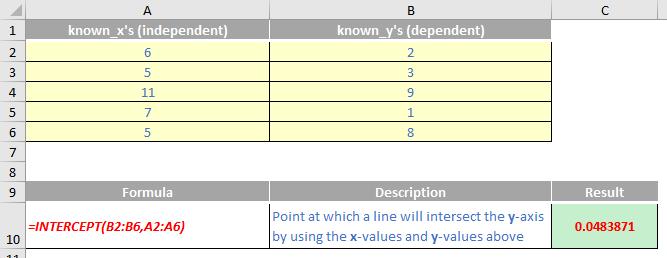
The INTERCEPT function calculates the point at which a line will intersect the y-axis by using existing x-values and y-values.  The intercept point is based on a best-fit regression line plotted through the known x-values and known y-values (as described above).  You should use the INTERCEPT function when you want to determine the value of the dependent variable when the independent variable is zero (0).  For example, you can use the INTERCEPT function to predict a metal's electrical resistance at 0°C when your data points were taken at room temperature and higher.

The INTERCEPT function employs the following syntax to operate:

The INTERCEPT function has the following arguments:

• known_y’s: this is required and represents the dependent set of observations or data
• known_x’s: this is also required and denotes the independent set of observations or data.

It should be noted that:

• if an array or reference argument contains text, logical values or empty cells, those values are ignored; however, cells with the value zero are included

• if known_y's and known_x's contain a different number of data points or contain no data points, INTERCEPT returns the #N/A error value

• The equation for the intercept of the regression line, a, is: 

where the slope, b, is calculated as:

and where x and y are the sample means AVERAGE(known_x's) and AVERAGE(known_y's)

• the underlying algorithm used in the INTERCEPT and SLOPE functions is different than the underlying algorithm used in the LINEST function. The difference between these algorithms can lead to different results when data is undetermined and collinear. For example, if the data points of the known_y's argument are zero (0) and the data points of the known_x's argument are one (1):
  • INTERCEPT and SLOPE return an #DIV/0! error. The INTERCEPT and SLOPE algorithm is designed to look for one and only one answer, and in this case there can be more than one answer
  • LINEST returns a value of zero (0). The LINEST algorithm is designed to return reasonable results for collinear data, and in this case at least one answer can be found.

Please see my example below:

We’ll continue our A to Z of Excel Functions soon. Keep checking back – there’s a new blog post every business day.

A full page of the function articles can be found here.