A to Z of Excel Functions: The IFS Function

Welcome back to our regular A to Z of Excel Functions blog. Today we look at the IFS function.

The IFS function

As a model developer and reviewer, I must confess I remain unconvinced about this one.  If you have ever used a formula with nested IF statements beginning with

then maybe this next function is for you – however, if you have ever written Excel formulas like this, then maybe Excel isn’t for you!  There are usually better ways of writing the formula using other functions.

Office 365 and Excel 2019 in all its variants has the relatively new function IFS.  The syntax for IFS is as follows:

IFS(logical_test1, value_if_true1, [logical_test2, value_if_true2], [logical_test3, value_if_true3],…)

where:

• logical_test1 is a logical condition that evaluates to TRUE or FALSE
• value_if_true1 is the result to be returned if logical_test1 evaluates to TRUE.  This may be empty
• logical_test2 (and onwards) are further conditions that evaluate to TRUE or FALSE also
• value_if_true2 (and onwards) are the respective results to be returned if the corresponding logical_test evaluates to TRUE.  Any or all may be empty.

Since functions are limited to 254 arguments (sometimes known as parameters), the new IFS function can contain 127 pairs of conditions and results.

One thing to note is that IFS is not quite the same as IF.  With the IF statement, the third argument corresponds to what do if the logical_test is not TRUE (that is, it is an ELSE condition).  IFS does not have an inherent ELSE condition, but it can be easily generated.  All you have to do is make the final logical_test equal to a condition which is always true such as TRUE or 1=1 (say).

Other issues to consider:

• whilst the value_if_true may be empty, it must not be omitted.  Having an odd number of arguments in an IFS statement would give rise to the “You’ve entered too few arguments for this function” error message
• if a logical_test is not actually a logical test (for example, it evaluates to something other than TRUE or FALSE, the function returns an #VALUE! error.  Numbers still appear to work though: any number than zero evaluates as TRUE and zero is considered to be FALSE
• if no TRUE conditions are found, this function returns the #N/A error.

To show how it works, consider the following example:

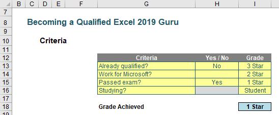
Here, would-be gurus are graded based on evaluation criteria in the table, applied in a particular order:

I think it’s safe that although it is reasonably straightforward to follow, it is entirely reasonable to say it’s not the prettiest, most elegant formula ever put to Excel paper.  In particular, do pay heed to the final logical_test: TRUE.  This ensures we have an ELSE condition as discussed above.

To be fair, one similar solution using previous Excel functions isn’t any better:

You may note I am not supplying multiple examples of IFS formulae.  This is because wherever possible you should try and replace the logic with a simpler, more accessible, logic for end users.  For instance, sometimes the logic of an elongated IF or IFS formula may be condensed to

In this situation, there is a function in Excel that can help.

My old English teacher said you should never start or finish a sentence with the word “and”.  AND is one of several Excel logic functions (others include NOT [already mentioned earlier, which takes the logical opposite of an expression] and OR). It returns TRUE if all of its arguments evaluate to TRUE; it returns FALSE if one or more arguments evaluate to FALSE.

One common use for the AND function is to expand the usefulness of other functions that perform logical tests.  For example, the IF function performs a logical test and then returns one value if the test evaluates to TRUE and another value if the test evaluates to FALSE.  By using the AND function as the logical_test argument of the IF function, you can test many different conditions instead of just one.

For example, imagine you are in New York on a Monday.  Consider the expression

where:

• condition1 is the condition, “today is Monday”
• condition2 is the condition, “you are in New York” and
• condition3 is the condition, “this author is the best looking guy you have ever seen”.

This would clearly be FALSE as not everywhere in the world it would be Monday (that is, condition1 would be breached)…

As alluded to above, the syntax for AND is as follows:

where:

• logical1: the first condition that you want to test that can evaluate to either TRUE or FALSE
• logical2: additional conditions that you want to test that can evaluate to either TRUE or FALSE, up to a maximum of 255 conditions. logical2 is optional and is not needed in the syntax.

It should be noted that:

• the arguments must evaluate to logical values, such as TRUE or FALSE, or the arguments must be arrays or references that contain logical values
• if an array or reference argument contains text or empty cells, those values are ignored
• if the specified range contains no logical values, the AND function returns the #VALUE! error value.

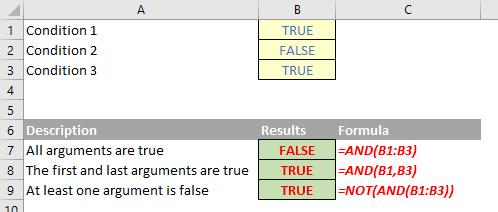
To highlight how AND works:

For a more practical example, consider the following summary data table:

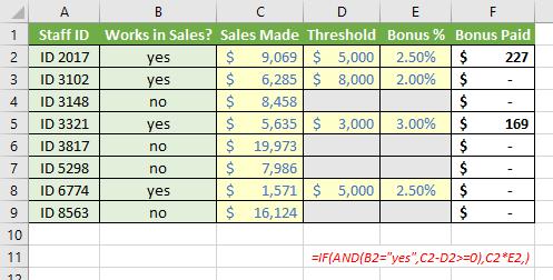
Here, we have a list of staff in column A, with identification of those who work in Sales (that is, eligible for a bonus) in column B.  Details of the sales made, the threshold for getting a bonus, and what rate it is paid are detailed in columns C, D, and E respectively.  The formula in cell F2:

denotes the Bonus Paid and is conditional on them working in Sales (B2="yes") and that the sales made were at or above the required threshold (C2-D2>=0).  If both conditions are TRUE, then a bonus (C2*E2) is paid accordingly (putting nothing after the final comma is the equivalent of saying “else zero”).  This is a prime example of IF and working together – and more often than not, these formulas are much easier to read than their IF(IF(IF or IFS counterparts.

The other logic function not yet mentioned, OR, is similar to AND, but only requires one condition to be TRUE.  Similar to AND, the OR function may be used to expand the usefulness of other functions that perform logical tests.  For example, the IF function performs a logical test and then returns one value if the test evaluates to TRUE and another value if the test evaluates to FALSE.  By using the OR function as the logical_test argument of the IF function, you can test many different conditions instead of just one.

For example, imagine you are in London on a Tuesday. Consider the expression

where:

• condition1 is the condition, “today is Tuesday”
• condition2 is the condition, “you are in London” or
• condition3 is the condition, “the Earth is flat”.

This would clearly be TRUE as you are definitely in London (that is, condition2 holds).

The syntax for OR is as follows:

where:

• logical1: the first condition that you want to test that can evaluate to either TRUE or FALSE
• logical2: additional conditions that you want to test that can evaluate to either TRUE or FALSE, up to a maximum of 255 conditions.  logical2 is optional and is not needed in the syntax.

It should be noted that:

• the arguments must evaluate to logical values, such as TRUE or FALSE, or the arguments must be arrays or references that contain logical values
• if an array or reference argument contains text or empty cells, those values are ignored
• if the specified range contains no logical values, the OR function returns the #VALUE! error value.

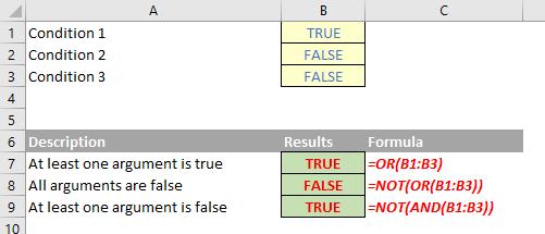
In summary, OR works as follows:

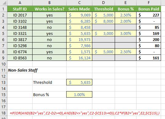
For a more practical example, consider the following summary data table:

Now there is a complex formula:

It isn’t quite as bad as it first seems. This is based on the AND case study from earlier, but it also allows for Non-Sales staff to participate in the bonus scheme too.  The logical_test in the primary IF statement,

Is essentially OR(condition1, condition2). The first condition is as before for Sales staff, whereas the second,

checks whether Non-Sales staff have exceeded the Non-Sales Staff threshold (cell C13).  Do you see that the check for Non-Sales staff is given by B2<>”yes” (B2 is not equal to ”yes”) rather than B2=”no”?  This takes me back to my earlier point about ensuring you develop your logical_test correctly.  It’s a subtle point, but will ensure all staff are considered (rather than excluding staff where no entry has been made in column B).

The other IF statement,

simply ensures the correct bonus rate is applied to the sales figure.

To summarise so far, sometimes your logical_test might consist of multiple criteria:

Here, this formula only gives a value of 1 if all three conditions are true.  This nested IF statement may be avoided using the logical function AND(Condition1,Condition2,…) which is only TRUE if and only if all dependent arguments are TRUE,

which is actually easier to read.  A similar example may be constructed for OR also.  However, even using these logic functions, formulas may become – or simply look – complex quite quickly.  There is an alternative: flags.  In its most common form, flags are evaluated as

condition=TRUE will give rise to a value of either TRUE or FALSE.  The brackets will ensure this is condition is evaluated first; multiplying by 1 will provide an end result of zero (if FALSE, as FALSE*1 = 0) or one (if TRUE, TRUE*1 = 1).  I know some modellers prefer TRUEs and FALSEs everywhere, but I think 1’s and 0’s are easier to read (when there are lots of them) and more importantly, easier to sum when you need to know how many issues there are.

Flags make it easier to follow the tested conditions.  Consider the following:

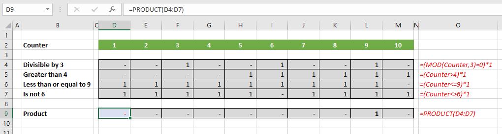
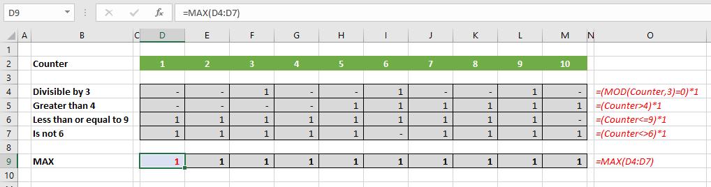
In this illustration, you might not understand what the MOD function does, but hopefully, you can follow each of the flags in rows 4 to 7 without being an Excel guru.  Row 9, the product, simply multiplies all of the flags together (using the PRODUCT function allows you to add additional conditions / rows easily).  This effectively produces a sophisticated AND flag, where all of the formulas are mercifully short.  If I wanted the flag to be a 1 as long as one of the above conditions is TRUE (that is, I wish to construct an OR equivalent), that is easy too:

Flags frequently make models more transparent and this example provides a great learning point.  Often, we mistakenly believe that condensing a model into fewer cells makes it more efficient and easier follow.  On the contrary, it is usually better to step out a calculation.  If it can be followed on a piece of paper (without access to the formula bar), then more people will follow it.  If more can follow the model logic, errors will be more easily spotted.  When this occurs, a model becomes trusted and therefore is of more value in decision-making.

Ne careful though. Sometimes you just can’t use flags.  Consider the following instance:

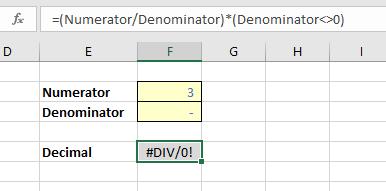
Here, the flag does not trap the division by zero error.  This is because this formula evaluates to

which equals #DIV/0! If you need to trap an error, you must use an IF function.

We’ll continue our A to Z of Excel Functions soon.  Keep checking back – there’s a new blog post every business day.

A full page of the function articles can be found here.