A to Z of Excel Functions: The HYPERLINK Function

Welcome back to our regular A to Z of Excel Functions blog.  Today we look at the HYPERLINK function.

The HYPERLINK function

I commonly use hyperlinks in my Excel files as they are a great way to move around a file.  If you create a central worksheet with hyperlinks to all of the other worksheets, you are only ever two clicks away from anywhere else in the workbook.  They make life very easy for end users and once you know how to construct them, they take mere seconds to insert.

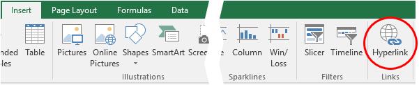
The ‘Insert Hyperlink’ dialog box is fairly straightforward to use and readily accessed via one of two keyboard shortcuts, either ALT + I + I or CTRL + K.  Alternatively, from the Ribbon, select the ‘Insert’ tab, click on ‘Hyperlink’ in the ‘Links’ group:

Hyperlinks can be used to link to a variety of places, but in this instance, I will focus on linking to elsewhere within the same workbook.

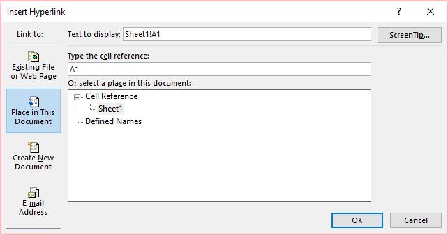
To create a hyperlink, first select the cell or range of cells that you wish to act as the hyperlink (i.e. clicking on any of these cells will activate the hyperlink).  Then, open the Insert Hyperlink dialog box (above) and select ‘Place in This Document’ as the ‘Link to:’, which will change the appearance of the rest of the dialog box. 

Insert the text for the hyperlink in the ‘Text to display:’ input box (clicking on the ‘ScreenTip…’ macro button will allow you to create an informative message in a message box when you hover over the hyperlink).

The next two input boxes, ‘Type the cell reference:’ and ‘Or select a place in this document:’, work in tandem – sort of:

• If you type a cell reference in the first input box without making a selection in the second input box, the hyperlink will link to the cell reference on the current (active) worksheet;
• If you type a cell reference in the first input box and select a worksheet reference in the second box, the hyperlink will link to the specified cell in the given worksheet.  In my example above, this hyperlink will jump to Sheet1 cell A1; or
• If you select a ‘Defined Name’ (i.e. a pre-defined range name) in the second input box, this will link to the cell(s) specified.  This is the recommended option, where available, if you wish to link to cell(s) on another worksheet within the same workbook.  This is because if the destination worksheet’s sheet name were to be changed, the link would still work.  I recommend that the range name should start with HL_ for Hyper Link, to make it easier to sort through range names if necessary.

It should be noted that there is an Excel function. I tend not to use this as it is not so user-friendly.  But let’s go through it anyway.  The HYPERLINK function creates a shortcut that jumps to another location in the current workbook, or opens a document stored on a network server, an intranet or the Internet.  When you click a cell that contains a HYPERLINK function, Excel jumps to the location listed, or opens the document you specified.  It employs the following syntax:

The HYPERLINK function syntax has the following arguments:

• link_location: this is required and represents the path and file name to the document to be opened.  The link_location can refer to a place in a document, such as a specific cell or named range in an Excel worksheet or workbook, or to a bookmark in a Microsoft Word document.  The path can be to a file that is stored on a hard disk drive.  The path can also be a universal naming convention (UNC) path on a server (in Microsoft Excel for Windows) or a Uniform Resource Locator (URL) path on the Internet or an intranet

It should be noted that on Excel for the web, the HYPERLINK function is valid for web addresses (URLs) only.  The link_location can be a text string enclosed in quotation marks or a reference to a cell that contains the link as a text string 

• If the jump specified in link_location does not exist or cannot be navigated, an error appears when you click the cell

• friendly_name: this argument is optional.  This is the jump text or numeric value that is displayed in the cell.  The friendly_name is displayed in blue and is underlined.  If friendly_name is omitted, the cell displays the link_location as the jump text

friendly_name may be a value, a text string, a name, or a cell that contains the jump text or value.  If friendly_name returns an error value (for example, #VALUE!), the cell displays the error instead of the jump text.

It should be noted that in the Excel desktop application, to select a cell that contains a hyperlink without jumping to the hyperlink destination, click the cell and hold the mouse button until the pointer becomes a cross, then release the mouse button.  In Excel for the web, select a cell by clicking it when the pointer is an arrow; jump to the hyperlink destination by clicking when the pointer is a pointing hand.

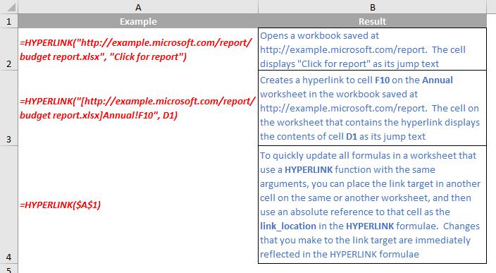
Please see my example below: 

We’ll continue our A to Z of Excel Functions soon.  Keep checking back – there’s a new blog post every business day.

A full page of the function articles can be found here.