
A to Z of Excel Functions: The GAUSS Function
27 January 2020
Welcome back to our regular A to Z of Excel Functions blog. Today we look at the GAUSS function.
The GAUSS function
Let’s start simply. Imagine I toss an unbiased coin: half of the time it will come down heads, half tails:

It is not the most exciting chart I have ever constructed, but it’s a start.
If I toss two coins, I get four possibilities: two heads, a head and a tail, a tail and a head, and two tails.

In summary, I should get two heads a quarter of the time, one head half of the time and no heads a quarter of the time. Note that (1/4) + (1/2) + (1/4) = 1. These fractions are the probabilities of the events occurring and the sum of all possible outcomes must always add up to 1.
The story is similar if we consider 16 coin tosses say:

Again, if you were to add up all of the individual probabilities, they would total to one (1). Notice that in symmetrical distributions (such as this one) it is common for the most likely event (here, eight heads) to be the event at the midpoint.
Of course, why should we stop at 16 coin tosses?

All of these charts represent probability distributions, i.e. it displays how the probabilities of certain events occurring are distributed. If we can formulate a probability distribution, we can estimate the likelihood of a particular event occurring (e.g. probability of precisely 47 heads from 100 coin tosses is 0.0666, probability of less than or equal to 25 heads occurring in 100 coin tosses is 2.82 x 10⁻⁷, etc.).
Now, I would like to ask the reader to verify this last chart. Assuming you can toss 100 coins, count the number of heads and record the outcome at one coin toss per second, it shouldn’t take you more than 4.0 X 10²²centuries to generate every permutation. Even if we were to simulate this experiment using a computer programme capable of generating many calculations a second it would not be possible. For example, in February 2012, the Japan Times announced a new computer that could compute 10,000,000,000,000,000 calculations per second. If we could use this computer, it would only take us a mere 401,969 years to perform this computation. Sorry, but I can’t afford the electricity bill.
Let’s put this all into perspective. All I am talking about here is considering 100 coin tosses. If only business were that simple. Potential outcomes for a business would be much more complex. Clearly, if we want to consider all possible outcomes, we can only do this using some sampling technique based on understanding the underlying probability distributions.
Probability Distributions
If I plotted charts for 1,000 or 10,000 coin tosses similar to the above, I would generate similarly shaped distributions. This classic distribution which only allows for two outcomes is known as the Binomial distribution and is regularly used in probabilistic analysis.
The 100 coin toss chart shows that the average (or ‘expected’ or ‘mean’) number of heads here is 50. This can be calculated using a weighted average in the usual way. The ‘spread’ of heads is clearly quite narrow (tapering off very sharply at less than 40 heads or greater than 60). This spread is measured by statisticians using a measure called standard deviation which is defined as the square root of the average value of the square of the difference between each possible outcome and the mean, i.e.
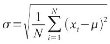
where: σ = standard deviation
N = total number of possible outcomes
Σ = summation
xi = each outcome event (from first x1 to last xN)
μ = mean or average
The Binomial distribution is not the most common distribution used in probability analysis: that honour belongs to the Gaussian or Normal distribution:

Generated by a complex mathematical formula, this distribution is defined by specifying the mean and standard deviation (see above). The reason it is so common is that in probability theory, the Central Limit Theorem (CLT) states that, given certain conditions, the mean of a sufficiently large number of independent random variables, each with finite mean and standard deviation, will approximate to a Normal (Gaussian) distribution.
The Normal distribution’s population is spread as follow:

i.e. 68% of the population is within one standard deviation of the mean, 95% within two standard deviations and 99.7% within three standard deviations.
The formula for the Normal distribution is given by
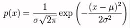
The GAUSS function calculates the probability that a member of a standard normal population will fall between the mean and z standard deviations from the mean. It has the following syntax:
GAUSS(z)
The GAUSS function has the following argument:
- z: this is required and this represents a number.
It should be noted that:
- if z is not a valid number, GAUSS returns the #NUM! error value
- if z is not a valid data type (i.e. it is not a number), GAUSS returns the #VALUE! error value
- because NORM.S.DIST(0,TRUE) always returns 0.5, GAUSS(z) will always be 0.5 less than NORM.S.DIST(z,TRUE).
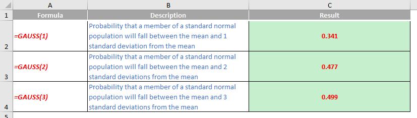
Please see my example below:
We’ll continue our A to Z of Excel Functions soon. Keep checking back – there’s a new blog post every business day.
A full page of the function articles can be found here.