A to Z of Excel Functions: The GAMMA.INV Function

Welcome back to our regular A to Z of Excel Functions blog.  Today we look at the GAMMA.INV function.

The GAMMA.INV function

The Gamma distribution is widely used in engineering, science and business, to model continuous variables that are always positive and have skewed distributions.  The Gamma distribution can be useful for any variable which is always positive, such as cohesion or shear strength for example. 

It is a distribution that arises naturally in processes for which the waiting times between events are relevant, and is often thought of as a waiting time between Poisson distributed events (the Poisson distribution is a discrete probability distribution that expresses the probability of a given number of events occurring in a fixed interval).  This is what is known as “queueing analysis”.

To understand it, first think of factorials, e.g. 5! = 5 x 4 x 3 x 2 x 1 = 120.  So far, so good, but how do you calculate if the factorial number you want to evaluate isn’t an integer?  The Gamma function is used to calculate this:

That’s great (if a little recursive), so can be expressed better (!) mathematically as follows:

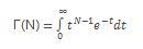
Clear as mud? Well, it gets better. The Gamma distribution just referred to has the following probability density function:

where ?(?) is the Gamma function, and the parameters ? and ? are both positive, i.e. ? > 0 and ? > 0:

• ? is known as the shape parameter, while ? is referred to as the scale parameter
• ? has the effect of stretching or compressing the range of the Gamma distribution. A Gamma distribution with ? = 1 is known as the standard Gamma distribution.

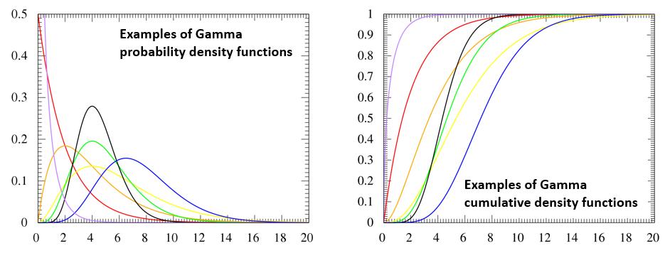
The Gamma distribution represents a family of shapes. As suggested by its name, ? controls the shape of the family of distributions. The fundamental shapes are characterized by the following values of ?:

• Case I (? < 1): when ? < 1, the Gamma distribution is exponentially shaped and asymptotic to both the vertical and horizontal axes
• Case II (? = 1): the Gamma distribution with shape parameter ? = 1 and scale parameter ? is the same as an exponential distribution of scale parameter (or mean) ?
• Case III (? > 1): when ? is greater than one, the Gamma distribution assumes a mounded (unimodal), but skewed shape. The skewness reduces as the value of ? increases.

The GAMMA.INV function is the inverse of the Gamma cumulative distribution, i.e. if p = GAMMA.DIST(x, ?, ?) then x = GAMMA.INV(p, ?, ?).  This can help to identify key points in a variable whose distribution may be skewed.  It has the following syntax:

The GAMMA.INV function has the following arguments:

• probability: this is required and this represents the probability associated with the distribution
• alpha: this is also required.  This is a parameter (the shape parameter) to the distribution
• beta: this too is  required and is another parameter (the scale parameter) to the distribution.  If beta = 1, GAMMA.DIST returns the standard gamma distribution.

It should be noted that:

• if any argument is text, GAMMA.INV returns the #VALUE! error value
• if probability < 0, if probability > 1, if alpha ? 0 or if beta ? 0, GAMMA.INV returns the #NUM! error value.

Given a value for probability, GAMMA.INV seeks that value x such that GAMMA.DIST(x, alpha, beta, TRUE) = probability.  Thus, the precision of GAMMA.INV depends upon the precision of GAMMA.DIST.  Therefore, GAMMA.INV uses an iterative search technique.  If the search has not converged after 64 iterations, the function returns the #N/A error value.

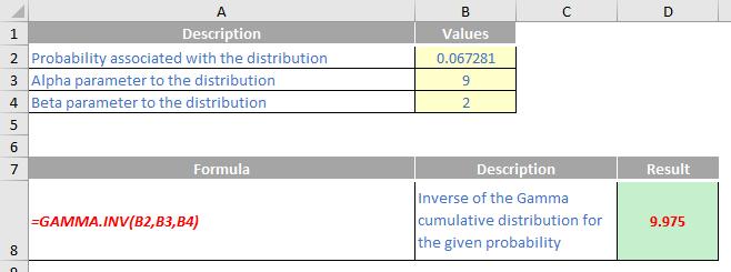
Please see my example below: 

We’ll continue our A to Z of Excel Functions soon. Keep checking back – there’s a new blog post every business day.

A full page of the function articles can be found here.