A to Z of Excel Functions: The F.TEST Function

Welcome back to our regular A to Z of Excel Functions blog. Today we look at the F.TEST function.

The F.TEST function

The F-distribution is defined as a continuous distribution obtained from the ratio of two chi-square distributions and used in particular to test the equality of the variances of two normally distributed variances a continuous probability distribution, which means that it is defined for an infinite number of different values.  This analysis of variance is often referred to as “ANOVA”, which I still think is a cheap car.

In slightly simpler terms, the F-distribution can be used for several types of applications, including testing hypotheses about the equality of two population variances and testing the validity of what is known as a multiple regression equation, i.e. a formulaic attempt to model the relationship between two or more explanatory variables and a response variable by fitting a linear equation to observed data.  

The F-distribution shares one important property with the Student’s t-distribution: probabilities are determined by a concept known as degrees of freedom.  Unlike the Student’s t-distribution, the F-distribution is characterized by two different types of degrees of freedom: numerator and denominator degrees of freedom.

The F-distribution has two important properties:

1. It’s defined only for positive values.
2. It’s not symmetrical about its mean; instead, it’s positively skewed.

A distribution is positively skewed if the mean is greater than the median (the mean is the average value of a distribution, and the median is the midpoint; half of the values in the distribution are below the median and half are above).  This function returns the (right-tailed) F probability distribution (degree of diversity) for two datasets.

This distribution is a relatively new one.  The associated F statistic is a ratio (a fraction). There are two sets of degrees of freedom; one for the numerator and one for the denominator.  As mentioned above, the F distribution is derived from the Student’s t-distribution. The values of the F distribution are squares of the corresponding values of the t-distribution.

To calculate the F ratio, two estimates of the variance are made:

1. Variance between samples: An estimate of ?² that is the variance of the sample means multiplied by n (when the sample sizes are the same).  If the samples are different sizes, the variance between samples is weighted to account for the different sample sizes.  The variance is also called variation due to treatment or explained variation
   
2. Variance within samples: An estimate of ?² that is the average of the sample variances (also known as a pooled variance).  When the sample sizes are different, the variance within samples is weighted.  The variance is also called the variation due to error or unexplained variation:

• SS_between = the sum of squares that represents the variation among the different samples
• SS_within = the sum of squares that represents the variation within samples that is due to chance.

To find a “sum of squares” means to add together squared quantities that, in some cases, may be weighted.  MS means “mean square”.  MS_between is the variance between groups, and MS_within is the variance within groups.

To calculate the sum of squares and the mean square, let:

• k = the number of different groups
• n_j = the size of the jth group
• s_j = the sum of the values in the jth group
• n = total number of all the values combined (total sample size: ?n_j)
• x = one value: ?x = ?s_j
• The sum of squares of all values from every group combined: ?x²

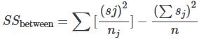
The between group variability is therefore

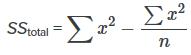
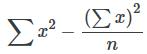
and the total sum of squares is given by

The explained variation is therefore the sum of squares representing variation among the different samples:

This should be compared with the unexplained variation, namely the sum of squares representing variation within samples due to chance, SS_within=SS_total?SS_between.

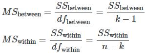
The degrees of freedom for different groups (i.e. the degrees of freedom for the numerator) is calculated as df = k – 1, whereas the equation for errors within samples (degrees of freedom for the denominator) is calculated as df_within = n – k.

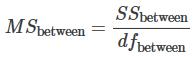
Further, the mean square (variance estimate) explained by the different groups is

whereas the mean square (variance estimate) that is due to chance (unexplained) is

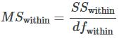
MS_between and MS_within can be written as follows:

The one-way ANOVA test depends on the fact that MS_between can be influenced by population differences among means of the several groups. Since MS_within compares values of each group to its own group mean, the fact that group means might be different does not affect MS_within.

The null hypothesis says that all groups are samples from populations having the same normal distribution. The alternate hypothesis says that at least two of the sample groups come from populations with different normal distributions. If the null hypothesis (H₀) is TRUE,
MS_between and MS_within should both estimate the same value.

To be clear, the null hypothesis says that all the group population means are equal. The hypothesis of equal means implies that the populations have the same normal distribution, because it is assumed that the populations are normal and that they have equal variances.

So, all of this brings us to the F-ratio or F-statistic, defined as

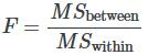
If MS_between and MS_within estimate the same value (following the belief that H₀ is TRUE), then the F-ratio should be approximately equal to one (1). Mostly, just sampling errors would contribute to variations away from one. As it turns out, MS_between consists of the population variance plus a variance produced from the differences between the samples. MS_within is an estimate of the population variance. Since variances are always positive, if the null hypothesis is FALSE, MS_between will generally be larger than MS_within. Then the F-ratio will be larger than one. However, if the population effect is small, it is not unlikely that MS_within will be larger in a given sample.

The foregoing calculations were done with groups of different sizes. If the groups are the same size, the calculations simplify somewhat, and the F-ratio can be written as:

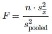
where

• n = the sample size
• df_numerator = k – 1
• df_denominator = n – k
• s²_pooled = the mean of the sample variances (pooled variance)
• S 2/x = the variance of the sample means.

Now that you have had the statistics lecture, you may use the worksheet function F.TEST to calculate an F-ratio on the data from two samples.  However, it does not return the F-ratio – no, that would be too simple.  Instead, it provides the two-tailed probability of the calculated F-ratio under H₀.  This means that the answer is the proportion of the area to the right of the F-ratio and to the left of the reciprocal of the F-ratio (i.e. 1 divided by the F-ratio).

Important: This function replaces the older function FTEST so that it may provide improved accuracy and whose names better reflect their usage.  Although the previous function is still available for backward compatibility, you should consider using this newer function from now on, because the older variant may not be available in future versions of Excel, according to Microsoft.

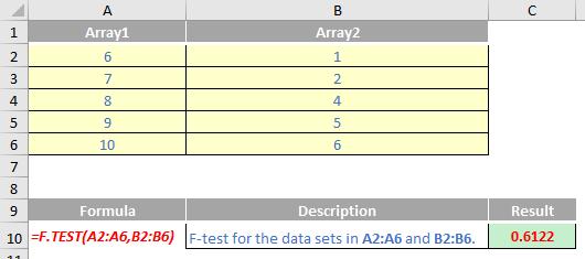
In summary, the F.TEST function returns the result of an F-test, i.e. the two-tailed probability that the variances in array1 and array2 are not significantly different.

The F.TEST function employs the following syntax to operate:

The F.TEST function has the following arguments: 

• array1: this is required and represents the first array or range of data
• array2: this is also required and denotes the second array or range of data.

It should be further noted that:

• the arguments must be either numbers or names, arrays or references that contain numbers
• if an array or reference argument contains text, logical values or empty cells, those values are ignored
• cells with the value zero will be included
• if the number of data points in array1 or array2 is less than two (2), or if the variance of array1 or array2 is zero, F.TEST returns the #DIV/0! error.

Please see my example below: 

We’ll continue our A to Z of Excel Functions soon. Keep checking back – there’s a new blog post every business day.

A full page of the function articles can be found here.