A to Z of Excel Functions: The BYCOL Function

Welcome back to our regular A to Z of Excel Functions blog.  Today we look at the BYCOL function.

The BYCOL function

BYCOL is not a region of the Philippines, but rather a function that takes an array or range and calls a lambda, with all the data grouped by each row or column and then returns an array of single values.

Its syntax is as follows:

It has the following arguments:

•  array: this is required, and represents an array to be separated by column
• lambda: an optional argument, this is a LAMBDA that takes a column as a single parameter and calculates just one result.

As an example, let’s discuss the weather – in particular, whether we use Celsius or Fahrenheit as our temperature scale.  I am based in Australia, so apologies to those in the United States, because I have made up some average monthly temperatures for Melbourne (Australia):

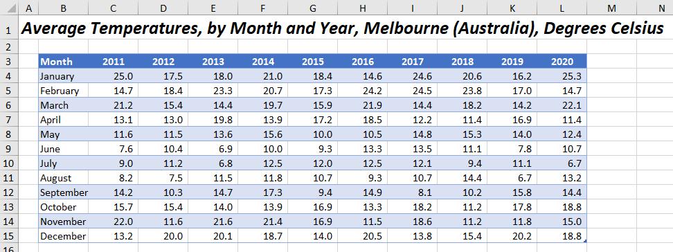
I have called this Excel Table Temps, but it is a permanent name…

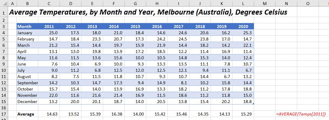
For the years 2011 to 2020 inclusive, I want to provide a detailed monthly breakdown of temperatures where the average temperature for the year was above 15 degrees Celsius.  At this point, you would normally calculate the average temperature for each column using a formula such as

for column C of this example spreadsheet.

This would be a “helper row”, e.g.

But I am not going to do it that way.  Instead, let’s use BYCOL.  First of all, let’s see how it works.  Consider the calculation

Here, we use the LAMBDA function to effectively create a user defined function to sum a column.

Note I have used Temps as my array, which is cells B4:L15, i.e. it omits the header row of the table (cells B3:L3).  I have to ignore the headers because the years would be included in the column totals being numbers – a classic gotcha!

This would produce the following result:

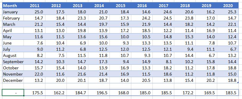
BYCOL produces a row vector, summing up each column of the table Temps, excluding the header row.  The formula spills, using dynamic array logic and matches the width of the underlying array (i.e. the Table Temps).  It only produces one row of data, as we have created a summation (just one value to report for each column).

Now, let’s consider the following formula:

Here, BYCOL produces a row of TRUE or FALSE values, depending upon whether the average for each column exceeds 15 degrees Celsius.  The dynamic array function FILTER, one of the recently introduced dynamic array functions then filters each column in Temps based upon whether the corresponding LAMBDA equates to TRUE or FALSE, viz.

This returns the columnar data for the years 2013, 2014, 2016, 2017 and 2020 respectively – not that you would know from the above numerical dataset.  I really wanted the headings, but having numerical values in the Table header did not help my cause (it would have caused my averages to calculate incorrectly).  It is usually not a good idea to have numerical values in Table headers, and perhaps now you can understand why.

If I modify the Table’s headers as follows, I can now use the entire Table:

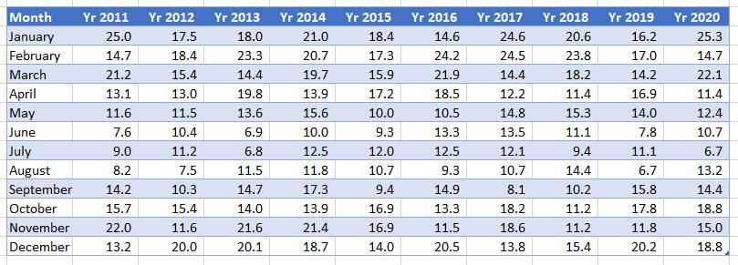
The formula may be modified to

which will produce a more informative spilled array:

We’ll continue our A to Z of Excel Functions soon.  Keep checking back – there’s a new blog post every other business day.

A full page of the function articles can be found here.