A to Z of Excel Functions: The AVERAGEIFS Function

Welcome back to our regular A to Z of Excel Functions blog.  Today we look at the AVERAGEIFS function.

The AVERAGEIFS function

Returns the average (arithmetic mean) of all cells that meet multiple criteria.  It is the “average” equivalent of SUMIFS.

The AVERAGEIFS function measures what is known as “central tendency”, which is the location of the centre of a group of numbers in a statistical distribution.  There are three common measures of central tendency:

• Average: the arithmetic mean, calculated by adding a group of numbers and then dividing by the count of those numbers.  For example, the average of 2, 3, 3, 5, 7, and 10 is 30 divided by 6, which is 5
• Median: the middle number of a group of numbers; that is, half the numbers have values that are greater than the median, and half the numbers have values that are less than the median.  For example, the median of 2, 3, 3, 5, 7, and 10 is 4.  If the number of values in the selection is an even number, the median is defined as the midpoint between the two central numbers
• Mode: the most frequently occurring number in a group of numbers.  For example, the mode of 2, 3, 3, 5, 7, and 10 is 3.

For a symmetrical distribution of a group of numbers, these three measures of central tendency are all the same.  For a skewed distribution of a group of numbers, they can be different.

The AVERAGEIFS function employs the following syntax to operate:

The AVERAGEIFS function has the following arguments:

• average_range: this is required.  One or more cells to average, including numbers, names, arrays, or references that contain numbers
• criterion_range1: this is required, consisting of one or more cells to use for the criterion1 and can include numbers or names, arrays, or references that contain numbers
• criterion_range2,…: up to a further 126 ranges (with associated criteria) are optional
• criterion1: this is also required.  The criterion in the form of a number, expression, cell reference, or text that defines which cells are averaged.  For example, criteria can be expressed as 32, "32", ">32", "apples", B4 or “>=”&B4.
• criterion2, ...: this is required if the corresponding optional criterion_range is invoked.  Syntax should be similar to that used for criterion1.

It should be further noted that:

• If average_range is a blank or text value, AVERAGEIFS returns the #DIV0! error value
• If a cell in a criteria range is empty, AVERAGEIFS treats it as a zero value
• Cells in range that contain TRUE evaluate as 1; cells in range that contain FALSE evaluate as zero
• Each cell in average_range is used in the average calculation only if all of the corresponding criteria specified are TRUE for that cell
• Unlike the range and criterion arguments in the AVERAGEIF function, in AVERAGEIFS each criterion_range must be the same size and shape as average_range
• If cells in average_range cannot be translated into numbers, AVERAGEIFS returns the #DIV0! error value
• If there are no cells that meet all the criteria, AVERAGEIFS returns the #DIV/0! error value
• You can use the wildcard characters, question mark (?) and asterisk (*), in criteria.  A question mark matches any single character; an asterisk matches any sequence of characters.  If you want to find an actual question mark or asterisk, type a tilde (~) before the character.

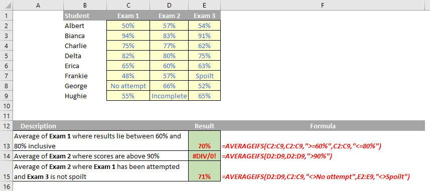
Please see my example below: 

We’ll continue our A to Z of Excel Functions soon.  Keep checking back – there’s a new blog post every other business day.