Time for Payback

In these uncertain times it is more important than ever to keep track of your cashflow.  Concentrating solely on profits may prove to be a fool’s game when cash rules the proverbial roost.  But to make money, you have to spend money – so how soon do you get it back?

That’s the topic for today’s article, where we look at the length of time it takes to recoup initial investment(s) and get back into the black.  How do you calculate the payback period in Excel such that it will be versatile to account for irregular periodicities, payment profiles and possible further outlays?

Let’s consider the following awkward example:

I have imagined some sort of infrastructure project with cash inflows and outflows on specific dates (e.g. they may have been stipulated by a contract).  Other than making the start date 1 January, I don’t think anyone will accuse me of creating a simple periodic example!

This is what motivated me to write on this topic.  All the solutions I ever see have regular, periodic cash flows with an outflow followed by inflows.  And yes, I have fallen for the latter trap – but I shall return to that subject in a short while.

To work out payback, I need two things:

1.      a running (cumulative) total of the overall cash flow

2.      an understanding of timing of the cash flows.

Therefore, I add two computations (all calculations are detailed in the attached Excel file):

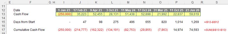
Calculating the timing of each cash flow is simple:

This formula simply subtracts the start date (I12) from the date of the particular cashflow on row 12.  For example, the third cash flow occurs on 9 April 2023, which is 98 days after the start date of 1 January 2023, etc.

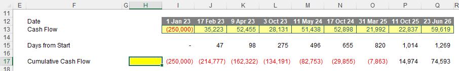
The cumulative cashflow is nothing more than a challenge of anchoring cell references correctly.  For example, the formula in cell I17 is given by

Again, column I is anchored, with all cashflows summed from the first period onwards.

We simply need to ascertain payback.  Many define this as when the cashflow first becomes non-negative (i.e. greater than or equal to zero [0]).  Consequently, many model using COUNTIF to calculate how many negative periods there are.  I disagree with this approach for two reasons:

1.      this methodology often assumes periods are equal in length (often, like in my above example, this is simply not the case)

2.      this logic fails to consider if there are any further outflows later when payback may have already occurred (e.g. material maintenance capital expenditure).  This can lead to entirely erroneous results, regardless of any regularity of periodicity considerations.

Therefore, I will not do it this way.  I want to know when the firstnon-negative period occurs.  This will provide my initial payback period, which is what I intend to calculate here.  It will not be distorted by any future negative cashflows.  I can determine this using the formula 

Here, the MATCH function considers the range $I$17:$Q$17 and assesses whether the values are non-negative.  In this instance, this will be evaluated as

MATCH then seeks TRUE in this array and match_type zero [0] the third argument allows for locating the first occurrence in a sequence provided in any order.  Thus, the first TRUE occurs in the eighth position, hence eight [8] is returned, i.e. 

Therefore, we now know that breakeven occurs afterthe seventh period but sometime up to or equal to the date of the eighth period.  The aim is to find at what point in this time interval, and to do this, I need one of my favourite functions I forever ramble on about, OFFSET.

OFFSET Recap

The oft-maligned OFFSET function considers disposition or displacement and has the following syntax:

The arguments in square brackets (height and width) may be omitted from the formula and are not germane to our problem today. 

In its most basic form, OFFSET(reference, rows, columns) will select a reference rows rows down (-rows would be rows rows up) and columns columns to the right (-columns would be columns columns to the left) of the reference.  For example, consider the following grid:

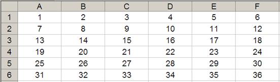
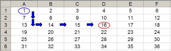
OFFSET(A1,2,3) would take us two rows down and three columns across to cell D3.  Therefore, OFFSET(A1,2,3) = 16, viz.

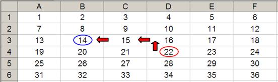
OFFSET(D4,-1,-2) would take us one row up and two rows to the left to cell B3.  Therefore, OFFSET(D4,-1,-2) = 14, viz.

This is especially useful when you wish to flex cell references.  Whilst functions such as INDEX may offer similar versatility, they require the full range to be known, whereas OFFSET does not.  Because position is stipulated rather than sought, OFFSET frequently calculates faster than INDEX; the reason OFFSET is not well liked amongst modelling academics is because it is a volatile function which means it often calculates when not needed (but not always!).  Quite frankly, this is not an issue in most spreadsheets modelled.  Indeed, in one 250+ MB file, our company noted that OFFSET calculated formulae up to 600 times faster.

Returning to Payback

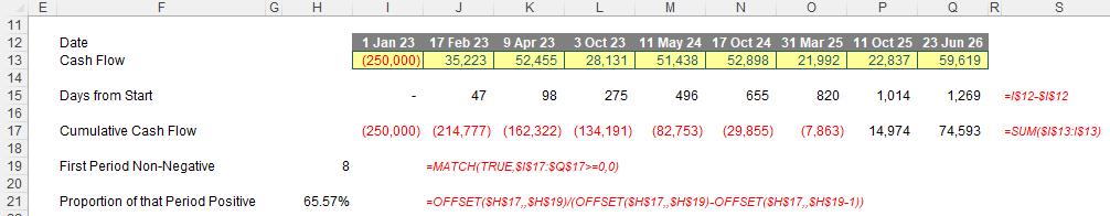
Assuming we have calculated the ‘First Period Non-Negative in cell H19 (see above), the proportion of that period that would be positive (strictly speaking, it would be non-negative) could be calculated as

This really is not as bad as it first looks.  Essentially, it is almost the same calculation no less than three times.  Consider the calculation

which is based upon cell H17:

This is the cell immediately to the left of the first cumulative cashflow.  Therefore, OFFSET($H$17,,$H$19) references the cell H19 – eight [8] – columns to the right of this cell, i.e. cell P17 which is the first non-negative cumulative cashflow ($14,974 for the date of 11 October 2025).

Similarly, OFFSET($H$17,,$H$19-1) returns the last negative cumulative cashflow seven [7] columns to the right of cell H17 in O17 ($(7,863) for the date of 31 March 2025).  Thus,

considers the increment in the cumulative cashflow for the eighth period.  Now, before everyone writes in and points out this is simply the value in cell P13 (which could have been derived using OFFSET($H$13,,$H$19)), I do realise this.  I am writing it this way to make the concept clearer.

Hence,

reflects the proportion of the cashflow for that period which puts the cumulative cashflow into surplus.  It also means that 100% less this proportion would represent the proportion of the period the cashflow remains in deficit.  But more on that anon. 

Now I have enough information to calculate the payback period in days:

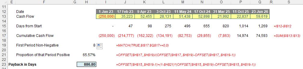
Here, in cell H23 I have constructed the formula

You may be already coming to terms with this formula now.  The first part

utilises a similar technique to the one described above by determining the total number of days up to and including the seventh start date (i.e. cell O15 which is 820 days).  

thus calculates the number of days between the seventh and eighth dates (i.e. P15 – O15 = 194 days).  This is analogous to the calculation for the cash for the eighth period constructed earlier.  This duration is then multiplied by 1-$H$21 to denote the duration of the period the cumulative cashflow remains negative.  Therefore, 

adds this proportion to the total number of days up to and including the last date.  This is the payback period in days.  I can divide this figure by the number of days in a year to present this duration in years if I wish (check out the Excel file for this final step).

Word to the Wise

Some of you will be noting the above, but feel uncomfortable that the time value of money has not been considered.  But this is a minor adjustment to the above technique.  All you do is calculate the present values of the cashflows first and then total these to construct the cumulative discounted cashflow.  The rest of the approach then ensues.

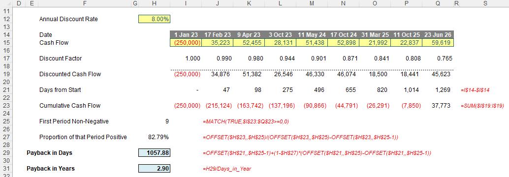
For those that feel a little nervous pro-rating periods linearly in this scenario, I completely understand – especially if the duration between dates is excessive.  However, this is what is done in practice and sometimes it is best to follow the flock.

Having said that, I address this consideration in calculating the optimisation of economic lives, but that is a story for another day…