Power Query: Aggregating Aggravating Worksheets

Welcome to our Power Query blog. Today I look at combining data from tables in several Excel worksheets.

I begin in a workbook that contains three worksheets. Each of the worksheets has been populated with a table of expenses information:

The initial process in order to start getting data from these worksheets is to go to the ‘POWER QUERY’ tab and create a new blank query, as shown below:

In the Power Query Editor, in the formula bar at the top of the screen, I enter the following formula:

which will list tables (and would list named ranges and workbook connections) that I have in my workbook as follows:

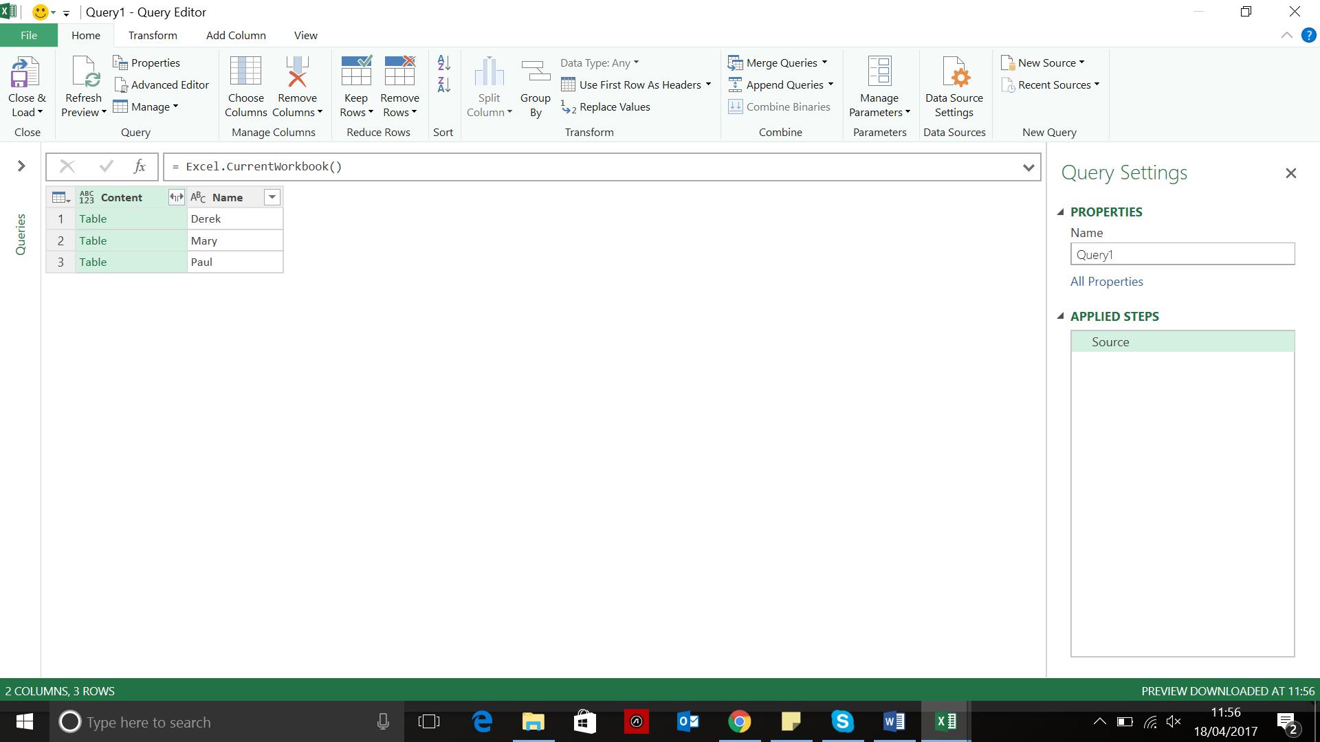
To keep it simple, my table names are the same as the worksheet names (note that this function will not extract data that is not in a table or named range). At this point, if I had other ranges or tables that I wanted to exclude from my query I could apply filters. The tables listed would include any connections from the workbook, and so this filter will be useful later. For now, I want all of my data, so the next step is to look at what the ‘Expand’ option next to the Content column title does:

I am given the option of selecting all of the columns from my tables. I don’t need to use the original column name as a prefix, so I uncheck that option. (There is also an option to ‘Aggregate’ instead of ‘Expand’, which is not appropriate for today’s example but this does deserve a blog entry of its own.) I choose to expand my data thus:

Now this data looks ready to load, so that’s what I will try next. All seems well to begin with, until I scroll down and find some unexpected data:

In order to see where this has come from, I go back to my query and check out my source step.

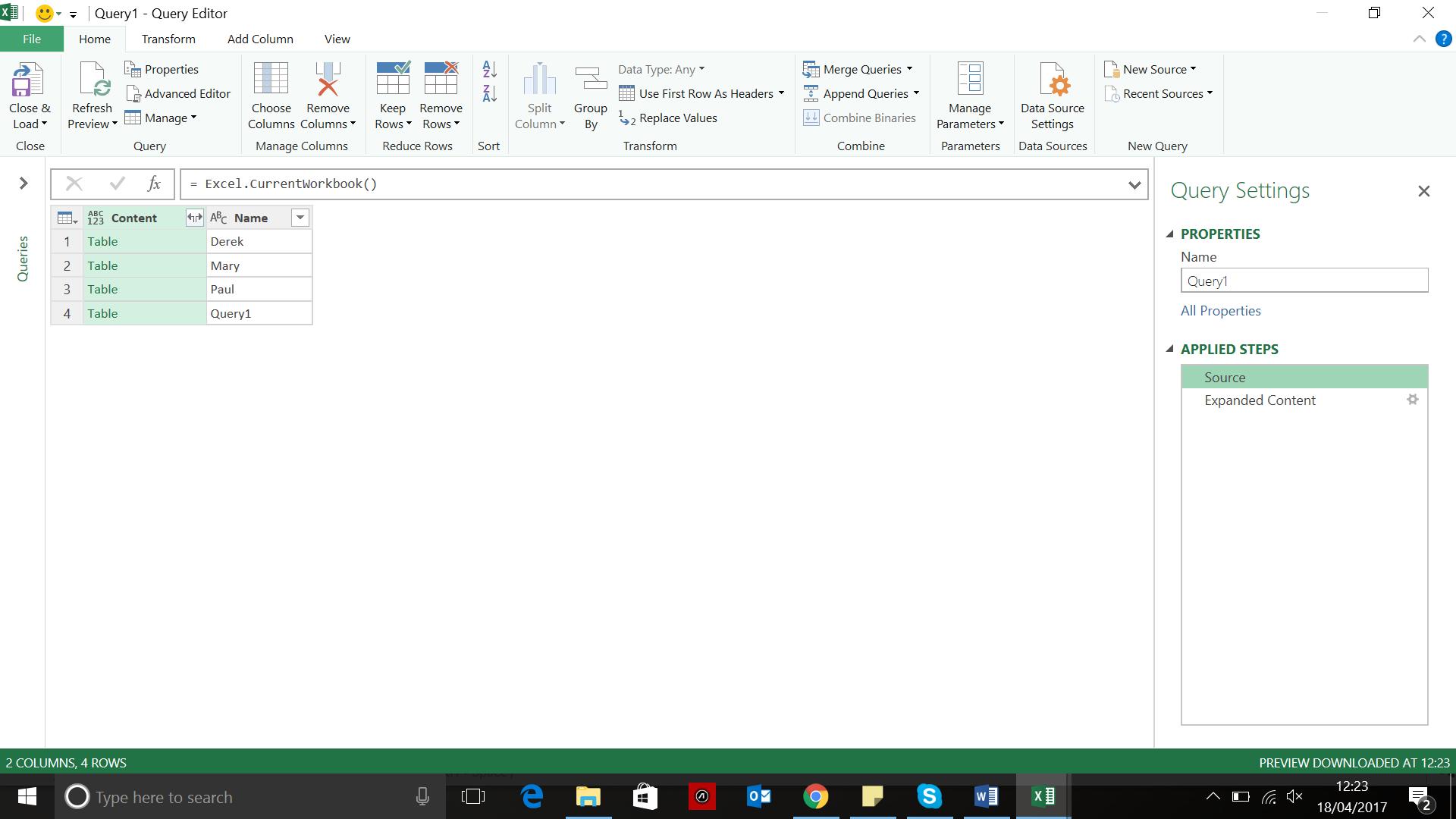
My query is a connection from the workbook, so it is included in the list of tables! Clearly, this is confusing my output, so I need to get rid of it from the source step. I can filter at this point and remove everything with the name ‘Query1’, but I will have to revise this if I change the name of my query. To show what I mean, I rename my query to ‘Expenses’ and review the options available in the filter of the ‘Source’ step:

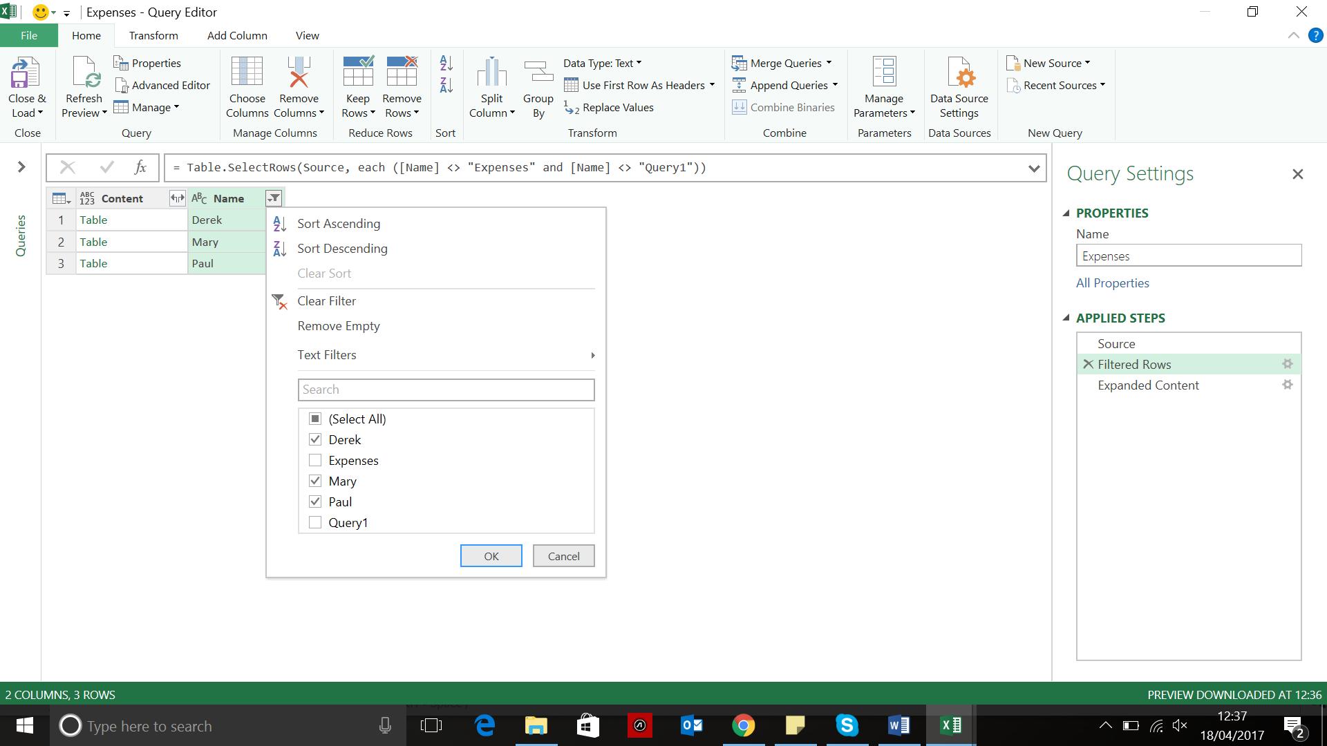
I filter out the Query1 and Expenses tables, and I am left with my expense data which can be uploaded:

Having chosen which ‘Name’ column to keep, my data appears on a separate worksheet to my other tables:

And so, I have my complete expenses list, with rather less rows uploaded this time. Next time I’ll have a look at how to pull in data from worksheets in other workbooks.

Want to read more about Power Query? A complete list of all our Power Query blogs can be found here. Come back next time for more ways to use Power Query!