
Knowing Your 2007 Times Tables
This article considers something that does not apply to Excel 2003 and earlier versions – Tables. By Liam Bastick, Director with SumProduct Pty Ltd.
Query
I understand Excel 2007 onwards has a Table functionality. Is this similar to Data Tables (see link)? Could you provide a brief overview for me?
Advice
With the release of Excel 2007, the Table functionality was introduced, superseding Excel 2003?s ‘List’ feature, in effect adding functionality. This has nothing at all to do with Data Tables.
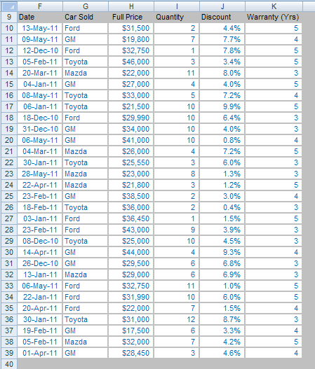
Creating a Table in Excel 2007 and later versions is straightforward, and simply requires the user to select the data to be used in the Table:
You do not even need to select the whole range: Excel will prompt for the whole Table even if only one cell is selected (PivotTable creation works similarly).
Next, from the Ribbon, in the ‘Styles’ group of the ‘Home’ tab, click on the button that says ‘Format as Table’:
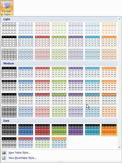
After clicking this button, Excel shows a new user interface element called a gallery, with a number of formatting choices for your Table, as displayed above. New styles may be created by selecting ‘New Table Style…’ if required.
After one of the formats has been chosen, Excel will prompt the user regarding which cells are to be converted to a Table:
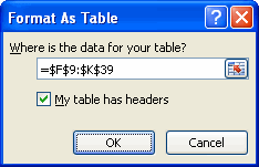
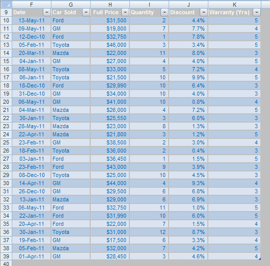
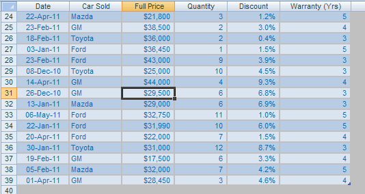
If the Table contains a heading row, ensure that the ‘My table has headers’ checkbox is checked. Click ‘OK’ to convert the range to a Table. Depending upon the selections made, a typical Table would look similar to the following:
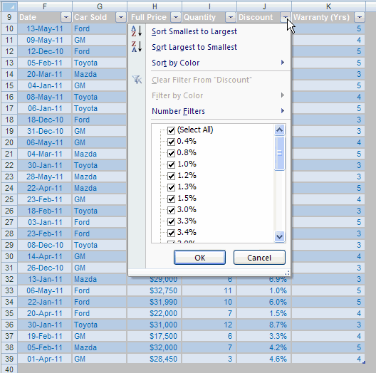
Tables have various useful functionalities, one such being the filtering which was done in lists in Excel 2003 and earlier versions. For example, provided the Table has a header row, it will always have in-built filter and sorting, which can be readily accessed from this top row.
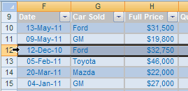
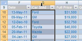
Selecting an entire column or row of a Table is similarly simple: the user just moves the mouse to the top of the Table or to the beginning of the first row until the pointer changes to a down or right pointing arrow, and then simply left-clicks. The data area of that column or row will be selected. For columns, the user should click again to include the header and any total rows in the selection.
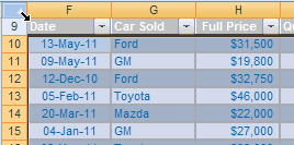
Furthermore, the whole Table can be selected in a similar fashion by positioning the mouse accordingly in the top left hand corner of the Table. The following diagrams illustrate these points.
Row
Column
All
One new quirk with the Table is the Frozen Header. Provided a cell has been selected within the Table, when users scroll down a Table such that the headers scroll off-screen, the column headings are temporarily replaced with the Table’s column names, insofar as the cursor is positioned within the Table, viz.
A Table will automatically resize to accommodate additional rows and / or columns, provided that data is entered in a cell immediately after the last column or row.
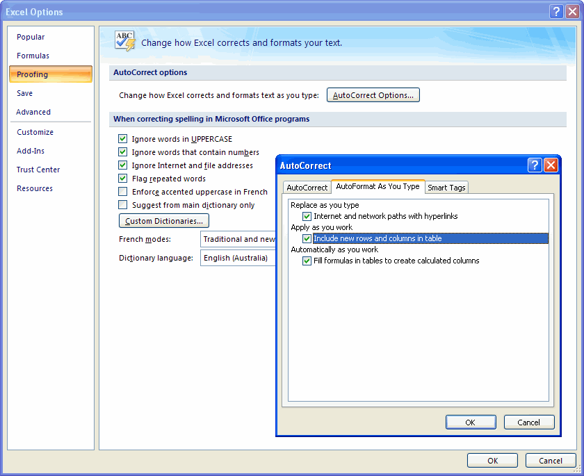
If Excel 2007 (or later) automatically adds a new row or column to the Table that is not required, click the ‘AutoCorrect Options’ button next to the expansion and then choose ‘Undo Table AutoExpansion’ from the drop down menu.
Also, it is possible to choose ‘Stop Automatically Expanding Tables’ from the drop down menu to turn off AutoExpansion. To turn it back on, use Office Button -> Excel Options -> Proofing -> AutoCorrect Options button (ALT + T + O + PP + [ALT & A]). In the AutoCorrect dialog box, click the ‘AutoFormat As You Type’ tab, select the ‘Include New Rows And Columns In Table’ check box, and then click the ‘OK’ buttons to close each dialog box in turn.
When a row or column is added / deleted in the Table, Excel 2007 will automatically adjust the formatting. For example, if alternate shading formatting has been chosen (as in the example above), this formatting will be retained.
If rows or columns are added to the Table, any object that uses the Table data will automatically include the new data. This will replace the need for dynamic range name creation (see link) often used in earlier versions that caused problems with some of Excel’s built-in functions. This makes adding data to charts very simple – just create the Table first for the chart data, and then add the chart in the usual way.
I strongly recommend naming Tables when working with multiple Tables. To do this, click on the Table and then from the ‘Table Tools’ -> ‘Design’ tab on the Ribbon, enter the Table Name in the Properties group as shown below (ALT + JT + A):

This Table Name is important as it is used when you refer to cells within the Table in a formula. For example, if you were to click in a cell immediately to the right of the Table, typed ‘=SUM(’ and then clicked on a cell within the Table, a formula similar to the following would appear:
=SUM(TableName[[#This Row],[Quantity]])
where:
- ‘TableName’ refers to the name given to the Table;
- ‘[# This Row]’ denotes that the data comes from the same row as the row that the formula is in; and
- ‘[Quantity]’ is the heading of the column referred to.
This gives rise to an important point regarding Table headings. Given their roles in Table reference formulae, no two columns may have the same heading. If a second heading is inadvertently given the same name as a prior one, Excel will automatically correct the duplication by appending a number to the new column name.
Also, once the formula is entered into the cell, the Table is automatically resized to include the formula (Excel puts in a default column heading as well, such as the imaginatively titled ‘Column1’) and the formula is automatically copied down to fill the entire column, consistent with the data. It is possible to undo these actions by using the smart tag that appears.
There’s more to Tables than this, but hopefully this provides a fair introduction (feel free to play with the attached Excel file). They are extremely versatile – as long as you are working in the more recent versions of Excel.