Sumproduct Squared..?
Finally we get round to our namesake! By Liam Bastick, Director with SumProduct Pty Ltd.
Query
I have been told by my colleagues that SUMPRODUCT is a very versatile Excel function. I am not sure I understand its full capabilities. Would you mind shedding some light please..?
Advice
SUMPRODUCT is one of my favourite Excel functions – hence the name of this company!
I have mentioned SUMPRODUCT in passing before (please see Multiple Criteria for more details). However, for the purposes of self-containment, let me recap on the basics first.
It should be noted that all of the examples below are included in the attached Excel file.
Basic Functionality
At first glance, SUMPRODUCT(vector1,vector2,…) appears quite humble. Before showing an example, though, look at the syntax carefully:
- A vector for Excel purposes is a collection of cells either one column wide or one row deep. For example, A1:A5 is a column vector, A1:E1 is a row vector, cell A1 is a unit vector and the range A1:E5 is not a vector (it is actually an array, but more on that later). The ranges must be contiguous; and
- This basis functionality uses the comma delimiter (,) to separate the arguments (vectors). Unlike most Excel functions, it is possible to use other delimiters, but this will be revisited shortly below.
Consider the following sales report:
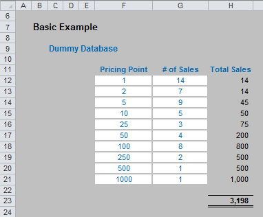
The sales in column H are simply the product of columns F and G, e.g. the formula in cell H12 is simply =F12*G12. Then, to calculate the entire amount cell H23 sums column H. This could all be performed much quicker using the following formula:
=SUMPRODUCT(F12:F21,G12:G21)
i.e. SUMPRODUCT does exactly what it says on the tin: it sums the individual products.

Dealing with Multiple Criteria
Where SUMPRODUCT comes into its own is when dealing with multiple criteria. This is done by considering the properties of TRUE and FALSE in Excel, namely:
- TRUE*number = number (e.g. TRUE*7 = 7); and
- FALSE*number = 0 (e.g. FALSE*7=0).
Consider the following example:
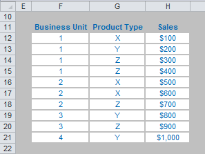
we can test columns F and G to check whether they equal our required values. SUMPRODUCT could be used as follows to sum only sales made by Business Unit 1 for Product Z, viz.
=SUMPRODUCT((F12:F21=1)*(G12:G21=”Z”)*H12:H21).
For the purposes of this calculation, (F12:F21=1) replaces the contents of cells F12:F21 with either TRUE or FALSE depending on whether the value contained in each cell equals 1 or not. The brackets are required to force Excel to compute this first before cross-multiplying.
Similarly, (G12:G21=”Z”) replaces the contents of cells G12:G21 with either TRUE or FALSE depending on whether the value “Z” is contained in each cell.
Therefore, the only time cells H12:H21 will be summed is when the corresponding cell in the arrays F12:F21 and G12:G21 are both TRUE, then you will get TRUE*TRUE*number, which equals the said number.
Notice that SUMPRODUCT is not an array formula (i.e. you do not use CTRL+SHIFT+ENTER, please see Array of Light), but it is an array function, so again it can use a lot of memory making the calculation speed of the file slow down.
Note also that this uses the * delimiter rather than the comma, analogous to TRUE*number, etc. If you were to use the comma delimiter instead, the syntax would have to be modified thus:
=SUMPRODUCT(–(F12:F21=1),–(G12:G21=”Z”),H12:H21).
Minus minus? The first negation in front of the brackets converts the array of TRUEs and FALSEs to numbers, albeit substituting -1 for TRUE and 0 for FALSE. The second minus sign negates these numbers so that TRUE is effectively 1, rather than -1, whilst FALSE remains equals to zero. This variant often confuses end users which is why I recommend the first version described above.
More Elaborate Uses
You can get more and more sophisticated:
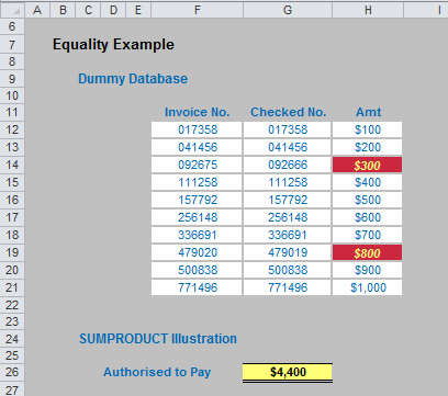
In this scenario, the end user pays invoices only where the invoice number matches the number “checked” on an authorised list. In the illustration above, two invoices (highlighted in red) do not match. SUMPRODUCT can be used to sum the authorised amounts only as follows:
=SUMPRODUCT((F12:F21=G12:G21)*H12:H21).
The argument in brackets only gives a value of TRUE for each row when the values in columns F and G are identical.
Another example includes neither the comma nor the multiplication delimiter:
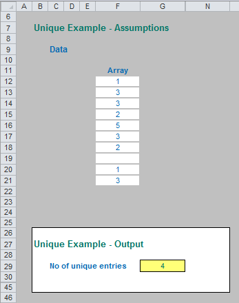
The formula in cell G29 in this illustration is:
=SUMPRODUCT((F12:F21<>“”)/COUNTIF(F12:F21,F12:F21&”")),
which is so intuitively clear there is no need for an explanation (!). Jokes aside, a full explanation can be found in the attached Excel file.
Comprehensive Example
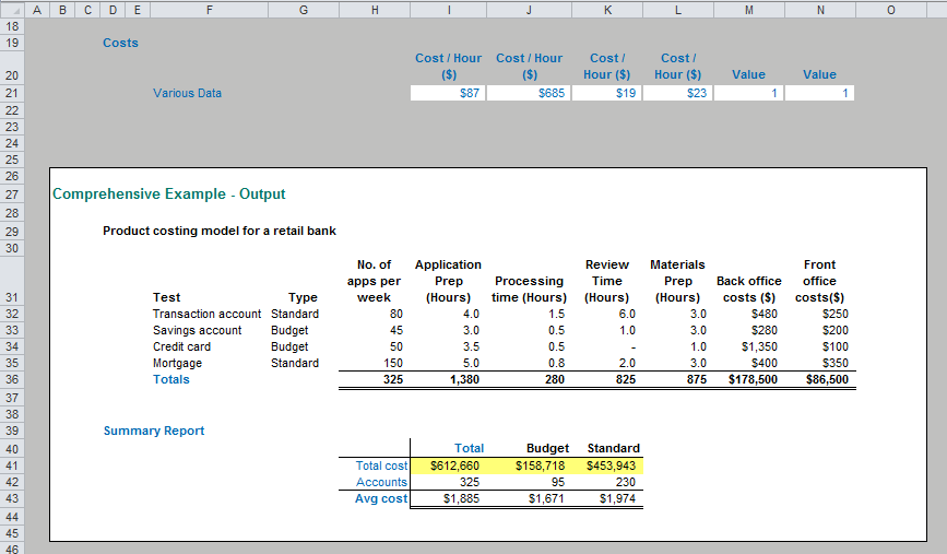
So far, I have only considered SUMPRODUCT with vector ranges. Using the multiplication delimiter (*), it is possible to use SUMPRODUCT with arrays (an array is a range of cells consisting of both more than one row and more than one column).
In the above example, SUMPRODUCT has been used in its elementary form in cells I36:N36. For example, the formula in cell I36 is:
=SUMPRODUCT($H$32:$H$35,I$32:I$35),
and this has then been copied across to the rest of the cells.
To calculate the total costs of this retail bank example, this could be calculated as:
=SUMPRODUCT($I$36:$N$36,$I$21:$N$21).
However, the formula in cell I41 appears more – and unnecessarily – complicated:
=SUMPRODUCT($H$32:$H$35*$I$32:$N$35*$I$21:$N$21).
The use of the multiplication delimiter is deliberate (the formula will not work if the delimiters were to become commas instead). It should be noted that this last formula is essentially
=SUMPRODUCT(Column_Vector*Array*Row_Vector),
where the number of rows in the Column_Vector must equal the number of rows in the Array, and also the number of columns in the Array must equal the number of columns in the Row_Vector.
The reason for this extended version of the formula is in order to divide the costs between Budget and Standard costs in my example. For example, the formula in cell J41 becomes:
=SUMPRODUCT($H$32:$H$35*$I$32:$N$35*$I$21:$N$21*($G$32:$G$35=J$40)),
i.e. the formula is now of the form
=SUMPRODUCT(Column_Vector*Array*Row_Vector*Condition),
where Condition uses similar logic to the TRUE / FALSE examples detailed earlier. This is a powerful concept that can be used to replace PivotTables (see >Pivotal PivotTables) for instance.
Word to the Wise
There are valid / more efficient alternatives to SUMPRODUCT in some instances. For example, dealing with multiple criteria for vector ranges, the SUMIFS function is six times faster, but will only work with Excel 2007 and later versions.
Over-use of SUMPRODUCT can slow the calculation time down of even the smallest of Excel files. Used sparingly, however, it can be a highly versatile addition to the modeller’s repertoire. It is a sophisticated function, but once you understand how it works, you can start to use SUMPRODUCT for a whole array of problems (pun intended!).

