
AGGREGATE: Sum of The Parts Are Confusing..?
This article reviews arguably the most complicated Excel function of them all: AGGREGATE. By Liam Bastick, Managing Director (and Excel MVP) with SumProduct Pty Ltd.
Query
Further to the SUBTOTAL function, Excel’s AGGREGATE function seems like an extension of SUBTOTAL. Do I have this correct?
Advice
AGGREGATE() is a relatively new Excel function, first emanating in Excel 2010. Therefore, it cannot be used in spreadsheets which may be opened in Excel 2007 or earlier as it will give rise to #NAME? errors.
For those who desire greater sesquipedalian loquaciousness (look it up!), its syntax may give some comfort as it has two forms:
- Reference: =AGGREGATE(Function_Number,Options,Ref1,[Ref2],…)
- Array: =AGGREGATE(Function_Number,Options,Array,[Optional_Argument])
where:
- Function_Number denotes function that you wish to use. Similar to SUBTOTAL, Function_Number allocates integer values to various Excel functions:

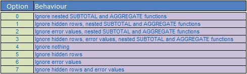
- Options specifies which values may be ignored when applying the chosen function to the range. If the Options parameter is omitted, the AGGREGATE function assumes that Options is set to 0. Options can take any of the following values:
- Ref1 is the first numeric argument for the function when using the Reference syntax
- Ref2,… is optional. Numerical arguments may number two through 253 for the function when using the Reference syntax
- Array is an array, array formula, or reference to a range of cells when using the Array syntax
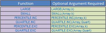
- Optional_Argument is a second argument required if using the LARGE, SMALL, PERCENTILE.INC, QUARTILE.INC, PERCENTILE.EXC or QUARTILE.EXC when using the Array syntax:
Our reader is quite right that AGGREGATE is analogous to an extension of the SUBTOTAL function insofar that it uses the same Function_Number arguments, simply adding another eight. SUBTOTAL allows users to use the 11 functions including / excluding hidden rows which results in 22 combinations. AGGREGATE goes further and takes the 19 functions and allows for eight alternatives for each, which results in 152 combinations – and that’s not even considering the Reference or Array syntax approaches!
It just all sounds, well, tremendously complicated.
Example
In practice, it’s not that bad. This is because since this function was created for Excel 2010 and later, screen tips will appear as you type in order to nudge you in the right direction. For example, let’s say you wanted the third largest number in the following list:

From inspection, the third largest value is the amount in cell A2 (the value ’5?), but if you use the usual formula for this =LARGE(A2:A10,3) you will get the value #REF! as this is the first error that Excel comes across as it works down the list.
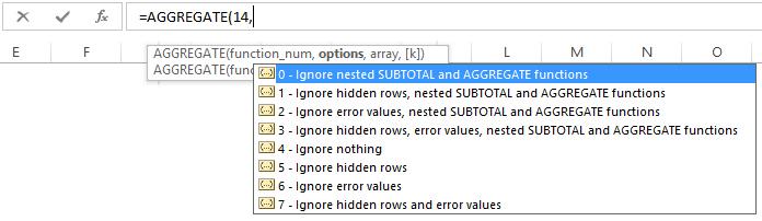
This is where you can use AGGREGATE() to ignore these errors. If you type in =AGGREGATE( you will get the following screen tip scroll list:

By typing ’14? or selecting ’14 – LARGE’ from the pop-up list, you now know you are on the right track. After typing a comma, Excel then continues to help you:
Again by either typing a number or pointing and clicking an appropriate choice may be made. I want to ignore errors, so I need to choose ’2?, ’3?, ’6? or ’7?, depending upon what else should be ignored. I will choose ’6? – ignore error values only and then type another comma so that the screen tips keep coming thick and fast:
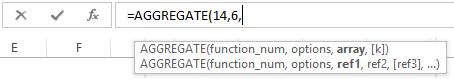
Now, Excel is seeking the references for evaluation. It appears to be possible that this can be in the form of a list (the array) or else discrete cell references and / or values. In this example, I will enter the range and type another comma:
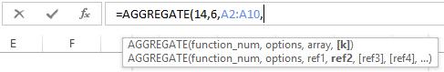
Now, Excel appears to be looking for the other argument for LARGE() or else another reference. This is not correct. The screen tip does not update automatically. The syntax required is now just as it would if we had typed in the underlying function, i.e. =LARGE(Array,k). In this instance, this syntax always requires the fourth value to be k, the integer denoting the kth largest item in the list.
In this example, I will just type the value ’3? and close brackets. Therefore, we arrive at the following formula,
=AGGREGATE(14,6,A2:A10,3)
which generates the correct answer ’5?. The formula might look counterintuitive, but Excel has helped us every step of the way. As my oft-misquoted English teacher always used to say, practice makes prefect.
Word to the Wise
Like SUBTOTAL, the AGGREGATE function is designed for columns of data (vertical ranges), not for rows of data (horizontal ranges). For example, when you subtotal a horizontal range using option 1, such as AGGREGATE(1, 1, Ref1), hiding a column does not affect the aggregate sum value, although hiding a row in vertical range does affect the aggregate.
If a second Ref argument is required but not provided, AGGREGATE returns a #VALUE! error.
If one or more of the references are 3-dimensional references, AGGREGATE returns the #VALUE! error value.
For more information, please inspect the attached Excel file.