Propose to Transpose Rows, I Suppose

What’s the best way to switch data from going across a row to down a column (or vice versa)? This article looks at the various ways of transposing data – and which way is probably “best”. By Liam Bastick, director with SumProduct Pty Ltd.

Query

I need to be able to transpose some formulae from rows to columns. What is the best way of doing this?

Advice

There are many occasions when data needs to be swapped between going across a row and going down a column (or vice versa), e.g. depreciation calculations (see An Appreciation of Depreciation for further details).

The question is, which approach should be used? Here, I look at four common methods.

Method 1: Cut and Paste a Formula

For the purposes of simplification, I am going to assume that we are looking to transpose data from going across a row to going down a column (the concepts are similar if columns are transposed into rows).

This method is very simple. First, create a formula that links to the data to be transposed, say, in the row beneath:

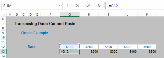
Second, once the formulae have all been created, cut and paste each formula individually into its appropriate position on the spreadsheet:

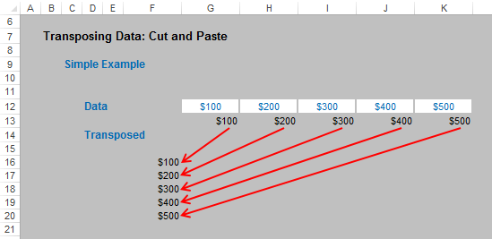
This is a very simple method, but certainly would be an ill-advised approach if you need to transpose 1,000 data points, for example.

However, simplicity is often a highly-underrated attribute in modelling. If you only have a few data items and you require the original inputs to remain (in our example, row 12, above), this method can often be deemed “simplest bestest”.

Method 2: Copy and Paste Special, Transpose

Another very simple approach is to copy and paste special as follows:

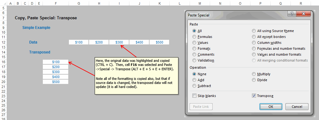
In this instance, simply highlight the data and copy the range in the usual way (e.g. CTRL + C). Next, simply select the first cell (i.e. the top left hand corner) of the intended range and Paste Special, Transpose (ALT + E + S + E + ENTER). As can be plainly seen from the illustration (above), the formatting as well as the content will be transposed.

This is an ideal approach for copying and transposing data from one source to another where links are not required. Aside from the inherited formatting, the main disadvantage here though is that depending upon the nature of the source data and how it is copied, updates in the original data will not flow through to the destination range.
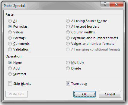
If the data needs to be linked to the source, then this approach is probably inappropriate. However, if inherited formatting is all that is putting you off, make the appropriate adjustments to the ‘Paste Special’ dialog box before pressing ‘OK’ / ENTER, e.g. set the dialog box as follows to copy only the formulae before transposing:

Method 3: Using the TRANSPOSE Function

On first glance, this looks like the “best” method. Once you discover there is a TRANSPOSE function, you think life is simple and your problems (well, you modelling problems anyway!) are over. Unfortunately, this function is not without its limitations.

Consider the following example:

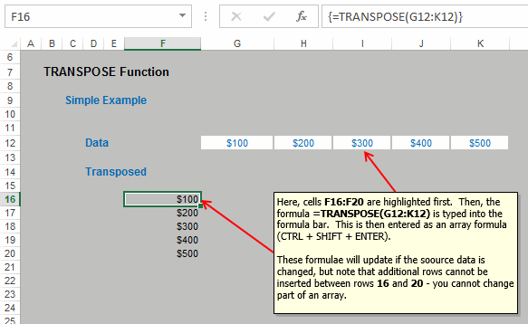
Here, the intention is to transpose the values in cells G12:K12 into the range F16:F20. To do this, simply highlight cells F16:F20 and then type in the following formula:

but rather than press ENTER, press CTRL + SHIFT + ENTER to enter the formula as an array formula instead (arrays have been discussed previously, see Array of Light for further details).

This method is very simple, as long as you ensure that the destination range contains precisely the same number of cells in the column as there are cells in the source row. If you change the source data, the outputs will update accordingly too.

So what’s the problem?

Array formulae can consume memory exponentially, which in turn can soon prevent Excel from calculating correctly, especially if you are working on a Windows 32-bit operating system, which is the platform most businesses employ.
Further, if you wanted to insert additional rows between rows 16 and 20 (e.g. to extend the range), you will find that this is not possible:

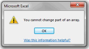
Only Chuck Norris can change part of an array, and unfortunately, he’s not available.

Interestingly, if you insert columns between G and K in the illustration above, this is possible, but the array formulae will not act like other Excel calculations: cell references in the TRANSPOSE formulae will not update (so the references will always link to what is in cells G12:K12 in our example). However, if you insert columns before column G, the formula will update. This can be confusing.

Therefore, TRANSPOSE is useful where you wish to protect the destination range’s structure, but it can be seen as inflexible and inefficient, particularly with larger Excel files, slowing calculation times down unnecessarily.

Method 4: OFFSET Approach

OFFSET is such a versatile function and has been discussed previously (see Onset of OFFSET). Used with the ROWS function (which simply counts the number of rows in a specified range), transpositions may be performed quickly and effectively using this method:

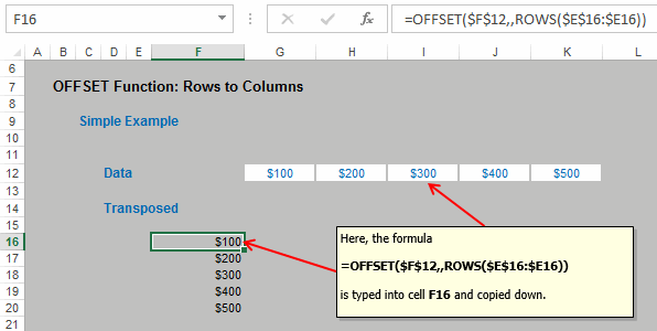
In this example, the following formula has been typed into cell F16:

As the formula is copied down, the number increases in the columns argument of OFFSET, as the number of rows increases. This is a neat trick for transposing without using array formulae, and can be seen as a good “general” solution, being quite flexible. The disadvantages here are twofold:

• Often modellers make mistakes in the absolute and semi-absolute references required to make this formula calculate correctly. This is easily overcome with practice; and
• The formula can look unnecessarily complex to the inexperienced or uninitiated. There are many end users (and modellers for that matter) unfamiliar with the OFFSET function in particular. It may be worthwhile to educate them accordingly.

These four examples (and a similar OFFSET example for transposing columns to rows) are all include in this month’s attached Excel file.

Word to the Wise

Astute readers will have noticed I have deliberately shied away from concluding which of the above four methods is “best”. This is because each of the four approaches has both pro’s and con’s. Personally, I would probably consign the TRANSPOSE function to the “functions only to be used in an emergency” category, but the other three options are not without their merits in certain situations – and their associated drawbacks.