Hiding Formulae
In this article we consider how to hide and protect formulae used in a spreadsheet. By Liam Bastick, Director with SumProduct Pty Ltd.
Query
I have been asked to put a spreadsheet together where users can neither view nor edit the formulae. Is this possible in Excel?
Advice
As with most things in Excel, there is more than one way to achieve a desired result. In this instance, the immediate solution appears to be to hide the Formula Bar in Excel as follows:
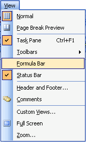
Excel 2003 and earlier
- Toggle the Formula toolbar on and off using View -> Formula Bar (ALT + V + F)
Excel 2007 and later
- Click on the ‘View’ tab on the Ribbon; and
- In the ‘Show / Hide’ group, check / uncheck the ‘Formula Bar’ check box as required
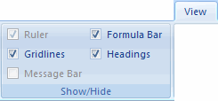
- ALT + V + F still works
This option might seem obvious and entirely reasonable at first, but there are issues with this approach:
- It is not just formulae that are ‘hidden’; no content can be viewed from the Formula Bar using this method;
- Formulae can still be viewed and edited by clicking on the cell in question and pressing the F2 (edit) function key; and
- The end user can simply switch the Formula Bar back on using the method(s) outlined above.
Now we may start to appreciate this seemingly simple query is not quite as straightforward as first thought. The problem here has three parts to it:
- How do we apply this to formulae only?
- How do we make sure it applies to all formulae?
- How can we prevent other users from undoing want we do and make formulae visible again?
Ensuring it Applies to Formulae Only
This method requires the formulae in Excel to be protected, whilst all other contents are not. All cells in Excel are ‘locked’ by default. This means that if the worksheet is protected, it will not be possible to edit these cells. We need to change this setting first of all.
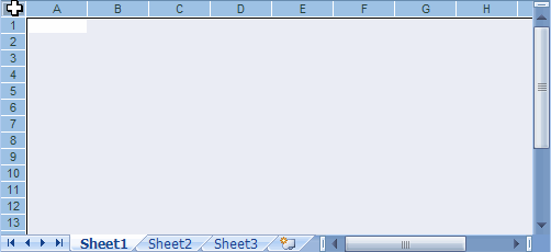
For each sheet that has formulae on that must neither be viewed nor edited, select all cells by either clicking on a blank cell and using the shortcut key CTRL + A or else select the box in the left hand corner between the row and column headers as so:
Next, Format Cells by using the shortcut key CTRL + 1 or ALT + O + E, go to the final tab (‘Protection’) of the ‘Format Cells’ dialog box and untick the ‘Locked’ check box shown below:

Click the ‘OK’ button. Repeat this process for each sheet. Now, if these sheets were to be protected, all cells could still be edited. This does seem to defeat the purpose of sheet protection, but the purpose of this initial step will become clear shortly.
Selecting All Formulae
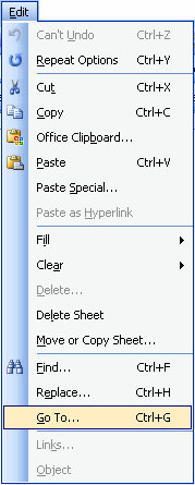
One of the most useful yet least used functionalities in Excel is the ‘Go To…’ feature. It may be activated as follows for each worksheet:
Excel 2003 and earlier
- Using the function key ‘F5’;
- Using the shortcut key CTRL + G; and
- Selecting Edit -> Go To… (ALT + E + G)
Excel 2007 and later
- Using the function key ‘F5’;
- Using the shortcut key CTRL + G; and
- Go to the ‘Home’ tab, ‘Editing’ group, click on the ‘Find & Select’ icon and choose ‘Go To…’ from the drop down menu
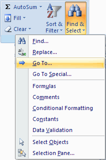
This brings up the ‘Go To…’ dialog box viz.
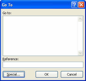
The trick here is then to select the ‘Special…’ button in the bottom left-hand corner (ALT + S). This brings up a further dialog box that many Excel users do not appear to be aware of, namely the ‘Go To Special’ dialog box:
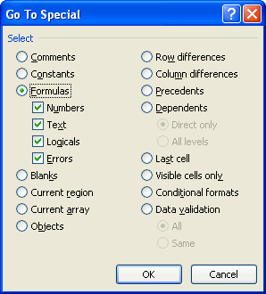
If we click on the ‘Formulas’ (sic) option button, and ensure the four check boxes remain ticked beneath it, this will ensure that all types of formulae (i.e. those containing hard code / numbers, text, logical operators and / or include errors such as #DIV/0!) will be selected on the worksheet once the ‘OK’ button has been depressed.
Now that all the formulae have been selected (the reader will note all of these cells are highlighted on the worksheet), we go back to the ‘Protection’ tab of the ‘Format Cells’ dialog box and change the settings as follows:
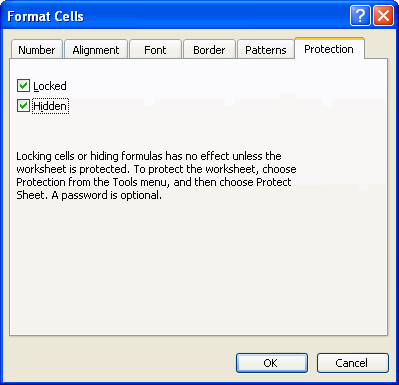
This time we tick both the ‘Locked’ and the ‘Hidden’ check boxes:
- ‘Locked’ will restrict these cells from being edited once the worksheet has been protected; and
- ‘Hidden’ will prevent the contents of these cells from being displayed in the Formula Bar once the worksheet has been protected.
This process needs to be repeated for each sheet, as required.
Sheet Protection
Finally, we have to protect each worksheet to stop users from simply reversing our changes. Sheet protection is enabled as follows:
Excel 2003 and earlier
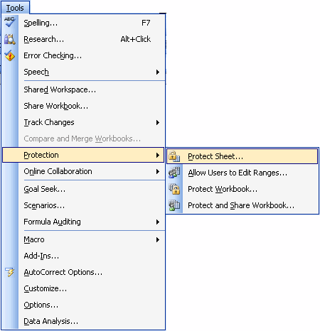
- Select Tools -> Protection -> Protect Sheet… (ALT + T + P + P)
Excel 2007 and later
- Click on the ‘Review’ tab on the Ribbon; and
- In the ‘Changes’ group, click on the ‘Protect Sheet’ icon

- ALT + T + P + P still works
This brings up the ‘Protect Sheet’ dialog box:
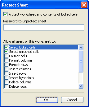
In older versions of Excel, this dialog box may appear slightly different, with only a password prompt displayed. Whether you employ a password or not is a personal preference, but if you want to ensure compatibility between all versions of Excel, only select the first two check boxes in the second window (headed ‘Allow all users of this worksheet to:’) (ALT + O).
Again, please repeat this process for each worksheet, as required.
Once this has been completed, formulae on this sheet will neither display in the Formula Bar nor be unlocked for editing, whilst all other cells will appear and function as they would in an unprotected sheet.

