Being Sensitive with Data Tables

In this article we show how to use one of Excel’s built-in features to undertake sensitivity analysis. By Liam Bastick, Director with SumProduct Pty Ltd.

Query

I understand Excel has a built-in feature, called Data Tables, that assists with sensitivity analysis. Could you explain how this functionality works please?

Advice

Just to be clear, when I refer to “sensitivity analysis” here, I mean the flexing of one or at most two variables to see how these changes in input affect key outputs. Excel has various built-in features that assist with this type of analysis. Here, we will focus on Data Tables.

Data Tables are ideal for executive summaries where you wish to show how changes in a particular input affect a key output. However, as always with modelling, Keep It Simple Stupid (KISS). If you can achieve the same functionality without using Data Tables in a simple, straightforward fashion, then do it that way. Consider the following example taken from the attached Excel file:

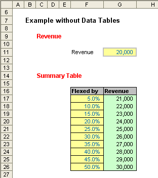
In this illustration, the key output revenue has been given in cell G11. We want to summarise what happens if we increase (“flex”) this figure by a given percentage, with the inputs specified in cells F17:F26. This can be simply computed by using the formula

in cell G17 and simply copying this calculation down.

Data Tables should really be used when such simple calculations are not possible and you want to flex one variable (known as a “one-variable” or “one-dimensional (1-D)” Data Table) or two (known as a “two-variable” or “two-dimensional (2-D)” Data Table).

I will now consider each in turn.

1-D Data Tables

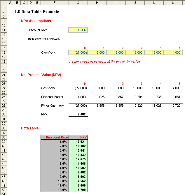
This is best illustrated using the following example – again from the attached Excel file.

Before readers write in, I appreciate this example could be constructed using a similar technique to our revenue example using the NPV function: I just wanted to construct a slightly more complex alternative that could still be followed!

Here, a simple Net Present Value is calculated for a total of six periods (0 to 5 inclusive). The output for a discount rate of 8.0% (cell G11) is +$9,482 (cell G30). But what if I wanted to know how the NPV would change if I varied the discount rate?

It is very easy to construct a table (a Data Table) similar to the one displayed in cells F38:G50 above. The required discount rates are simply typed into cells F39:F50, but the headings in cells F38:G38 are not what they seem.

For a 1-D Data Table to work using a columnar table similar to the one illustrated, the top row has to contain the reference to the input cell in the left hand cell (F38 must be ‘=G11’) and to the output cell in the right hand cell (G38 must be ‘=G30’). Many modellers will do this, putting the headings in the row above instead and then they may or may not hide row 38 in order to compensate.

There is a crafty alternative (employed above).

Using CTRL + 1 or ALT + O + E to Format Cells, if we go to the ‘Number’ tab we can still type the formulae in but change the outward appearance of the cell. For example, cell F38 is formatted as follows:

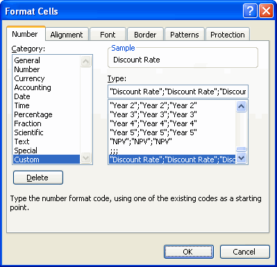
Here, I have typed in “Discount Rate”;”Discount Rate”;”Discount Rate”. Custom number formatting is explained in this link, but essentially this syntax forces Excel to display any numerical output as “Discount Rate”. Note that simply typing “Discount Rate” here once would be insufficient: e.g. if the output were negative, the cell would be displayed as “-Discount Rate”. G38 is formatted similarly.

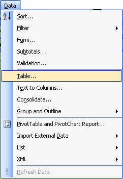
Once row 38 has been finalised, highlight cells F38:G50 and then create the Data Table:

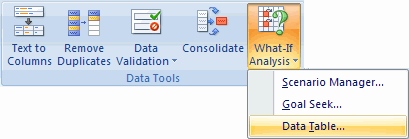
This gives rise to the following dialog box:

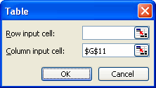
In a 1-D Data Table only one of these two input cells should be populated. When the table is of a columnar format, the column input cell should be populated, referring to the input cell, as above.

If the table had been across a row instead, ensure that the input value are in the top row, and that the ‘headings’ are in the first column (i.e. transpose the example table above). Then, you would populate the ‘Row input cell:’ box above instead.

Once ‘OK’ has been clicked, the Data Table will populate showing what the NPV would be for alternative discount rates. The formula should be noted: {=TABLE(,G11)} shows this is an array function with G11 as the column input cell. The use of array functions here means that once constructed, the Data Table may not be modified partially.

1-D Data Tables do not need to be simply two columns or two rows. It is entirely possible to display the effects on more than one output at the same time provided you wish to use the same inputs throughout the sensitivity analysis, viz.

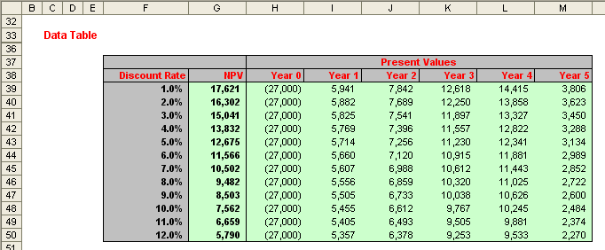
Please review the attached Excel file for further details.

2-D Data Tables

These Data Tables are similar in idea: they simply allow for two inputs to be varied at the same time. Let’s extend the 1-D example as follows (again referring to the attached Excel file):

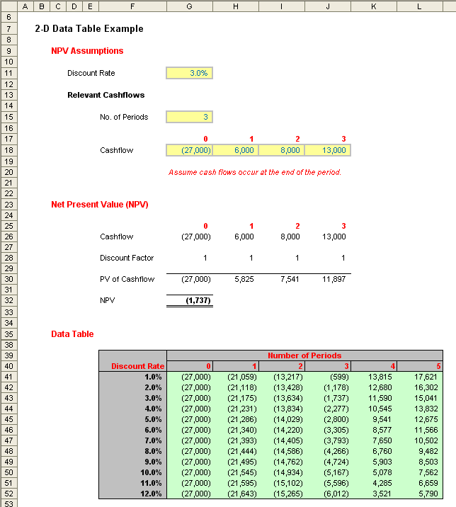
This example is similar, but only calculates the NPV for a certain number of periods – specified in cell G15. Our 2-D Data Table (which is cells F40:L52, not F39:L52) can answer the question, “What is the NPV of our project over x periods with a discount rate of y%?”.

If anything, a 2-D Data Table is simpler than its 1-D counterpart since there is little confusion over row and column input cells. Again, the output needs to be in the table, this time it must be in the top left hand corner of the array. In our example, it is disguised as “Discount Rate” using similar number formatting to that described earlier.

The inputs required now form the remainder of the top row and the first column of the Data Table. With cells F40:L52 highlighted, the Data Table dialog box is opened as before:

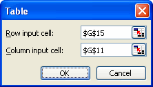
Since the top row are the inputs for the Number of Periods, the ‘Row input cell:’ should reference $G$15, whilst the discount rate inputs (‘Column input cell:’) should link to $G$11 once more.

Once ‘OK’ is depressed, the Data Table will populate as required – simple!

Important Considerations

Data Tables can be really useful for executive summaries, but there are drawbacks to consider:

• The variable inputs to be flexed should always be hard coded, since formulae do not work as envisaged with this feature. This can prove cumbersome if you wish to change the Data Tables regularly;
• There are workarounds, but in general, the inputs and outputs should be on the same worksheet as the Data Table. This is not always ideal and the alternative (beyond the scope of this article) may be perceived as convoluted;
• Data Tables can slow down the file calculation time dramatically. For example, if you have just three 2-D Data Tables, each with ten inputs on each axis, the model calculation time could increase by a factor of up to 300 (= 3 x 10 x 10);
• Microsoft has recognised this issue and allows you to change Excel’s Calculation option (found in ALT + T + O, under ‘Calculation’) to ‘Automatic except tables’. I strongly recommend you do not implement this option. End users tend to assume Excel is always calculating everything automatically and some do not know how to check / modify this functionality;
• Instead, I would build in ‘On / Off’ switches next to the Data Tables themselves. These are transparent and intuitive and have the same effect (please review the attached Excel file for how to build in this optionality); and finally
• Data Tables will only flex one or two variables at a time. If more variations are changed, consider using Excel’s Scenario Manager or the Solver add-in (depending upon your requirements, not discussed here).