Keeping Up Appearances: Conditional Formatting
This article discusses how to change the appearance of a cell and compares the new Excel 2007 features for conditional formatting. By Liam Bastick, director with SumProduct Pty Ltd.
Query
How can I change the appearance of cells based on their contents? Do I need to write a macro?
Advice
With Excel’s IF function, the contents of a cell can be modified depending upon (a) certain condition(s) being met (i.e. held to be TRUE). However, the formatting or style of the cell cannot be changed in this manner.
Macros are not needed.
Conditional Formatting is an Excel feature that does allow you to apply formats to a cell or range of cells, and have that formatting change depending on the value of the cell or the value of a corresponding formula.
This is one of the features that has been given a major overhaul in Excel 2007 and therefore to address today’s query, I am splitting my response in two: one for Excel 2007 and one for earlier versions.
Excel 2003 and Earlier
Conditional Formatting is accessed from the Format drop-down menu (Format -> Conditional Formatting… or ALT + O + D).

For conditional formatting to apply to a cell, the value in the cell must meet a certain condition or else a formula associated with the cell must be TRUE.
For example, in the following graphic, the cell will be coloured a delightful orange on pink (based on ‘Format’ settings selected after clicking on the said button) if the value is between the values contained in cells B1 and C1:

This could also be achieved with the “Formula Is” option as follows:

However, this assumes that the cell is A1, that B1 and C1 contain numbers and that B1 is less than or equal to C1. In this instance, it is much easier to use the “Cell Value Is” approach.
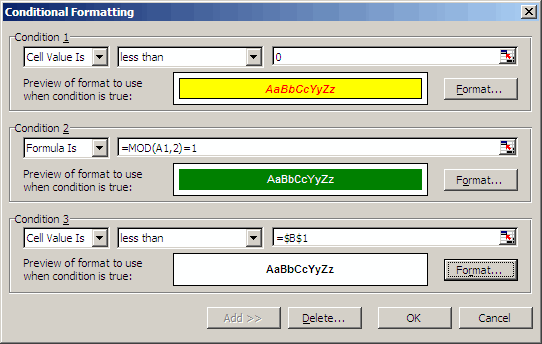
It is possible to define up to four mutually exclusive formats for any given Excel cell. This is achieved by clicking on the ‘Add’ button. Up to three conditions can be defined, viz.
With Excel 2003 and earlier versions, conditional formatting works as follows:
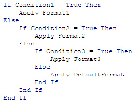
Essentially, as soon as Excel finds a condition that is held it formats accordingly and stops. If none of the three conditions is met, the underlying format (i.e. the fourth format) is retained.
In the three conditions illustration above, Excel will format as follows:
- If the value in the cell is less than zero, it will colour it bold red on yellow;
- If the value in the cell is greater than or equal to zero and odd, it will colour it white on green;
- If the value in the cell is greater than or equal to zero, even and less than the value input in cell B1, it will make the font bold; otherwise
- If the value in the cell is greater than or equal to zero, even and greater than or equal to the value in cell B1, the original formatting will be retained.
Note that if the value in cell B1 is less than zero and the value in the cell formatted is less than B1 and odd, technically, all three conditions are met. However, Excel stops once the first condition is met for Excel 03 and earlier versions – so the order the conditions are stipulated is important for this feature.
Excel 2007
Conditional formatting has been revamped and reinvented in Excel 2007. Located in the Styles group of the Home tab, the conditional formatting feature has had a raft of new features added.
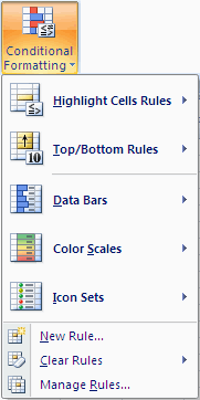
For instance, inspecting ‘Highlight Cells Rules’ is akin to many of the “Cell Value Is” functionalities of its predecessor, e.g. Greater Than, Less Than, Between, Equal To. However, new options are also available: Date Occurring and Duplicate Values. All you have to do is highlight the list, select the option and colour scheme required. Simple (no need to concoct hideous formulae such as
=IF(COUNTIF($A:$A,$A1)>1,COUNTIF($A$1:$A1,$A1)>1)
for locating duplicates, for example).
Users should not be fooled by the easy-to-use Top / Bottom Rules either. Top 10 Items, Top 10%, Bottom 10 Items and Bottom 10% all highlight items that conform to these labels. However, the ‘10’ can be changed to a number of the user’s choice. Who could possibly live without the Bottom 37% Debtors Report for instance… .
Above average and below average data can be highlighted also in one or two clicks. In Excel 2003, all of this functionality was available too, but not in one or two clicks. For example, to highlight the bottom 37%, the user would have to type a formula into “Formula Is” such as:
=Cell_Ref<=PERCENTILE(Range,0.37)
which requires the user knowing the PERCENTILE function (certainly not in the top 30 most commonly used functions).
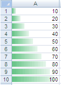
Excel 2007 allows graded shading of a cell as well. For example, if cells A1:A10 had the values 10, 20, 30, …, 100 respectively, the cells could be filled in as follows:
Excel 2003 and earlier
Excel 2007
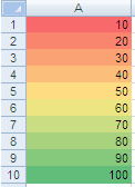
Clearly, looking at the Color Scales example, conditional formatting lends itself neatly to traffic light reporting. This is compounded by Icon Sets that will stratify data into between three and five sections using various icons (such as the red, amber and green traffic lights). Given that Excel 2007 now permits cells to be sorted dependent upon their background colour (ALT + D + S, then choose ‘Cell Color’ in ‘Sort On’ field), Excel 2007 can make monthly reporting a colourful adventure!
Data Bars, Color Scales and Icon Sets cannot be replicated in Excel 2003, so these are not backwards compatible. Furthermore, conditional formatting in Excel 2007 differs logically in one key way.
As explained in the ‘Excel 2003 and Earlier’ section (above), as soon as Excel finds a condition that is held it formats accordingly and stops. This can be performed for up three conditions. In Excel 2007, there is ‘no limit’ and testing does not have to stop (i.e. more than one format can be applied in a cell at a time), i.e.
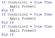
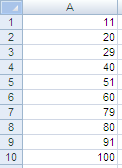
To highlight this, consider the following data set before and after multiple conditional formatting:
Before Multiple Conditional Formatting
After Multiple Conditional Formatting
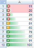
No less than four conditional formats have been applied, as can be seen by opening up the Conditional Formatting Rules Manager (ALT + O + D):
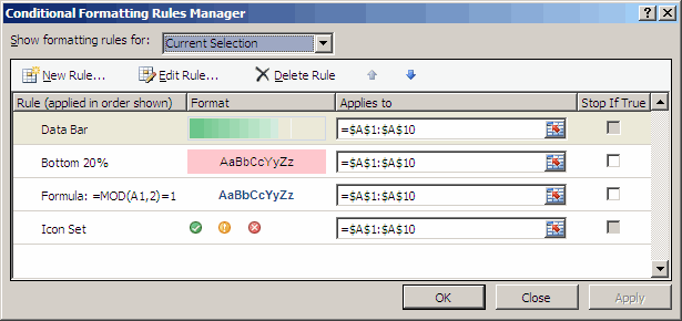
Using the blue up and down arrows can reorder the sequence and the sequence can be stopped if certain conditions are true (simply check the box in the fourth columns). This gives Excel 07 conditional formatting significantly greater flexibility than its earlier guises.
If you have a query for this section, please feel free to drop Liam a line at liam.bastick@sumproduct.com or visit the website www.sumproduct.com

