Avoiding a Group Protection Racket

Here, we address one of the most common questions raised in financial modelling: how can you group / un-group rows and / or columns when the worksheet is protected? By Liam Bastick, Director with SumProduct Pty Ltd.

Query

I need to protect my worksheet to avoid users typing over important calculations. However, I want the users to be able to group and un-group various rows and columns. Is this possible?

Advice

I have written about sheet protection previously (see Wearing Protection).

If you open any workbook and select any cell in any given worksheet, you will note that the cell is “locked” by default (simply go to the cell, then depress CTRL + 1 and select the ‘Protection’ tab), viz.

As the narrative in the dialog box notes, locking cells has no effect until the worksheet is protected. This is simple to prove: all cells are locked by default yet anyone can still edit any cell at will.

In order to protect the contents, you have to protect the worksheet (ALT + T + P + P in all versions of Excel, otherwise ‘Home’ tab of the Ribbon, then select ‘Format’ in the ‘Cells’ group and then select ‘Protect Sheet…’ in Excel 2007 onwards). For later versions of Excel, this will promote the following dialog box:

It is only when the sheet has been protected that locked cells are protected. Other actions may or may not be allowed by checking the various check boxes displayed above. The above image shows many of the options available (e.g. formatting cells, rows, columns, etc.).

However, one useful – and common feature missing is grouping…

Grouping

Sometimes when constructing spreadsheets modellers may want to hide certain data / calculations. This can be undertaken by formatting the cells (see Number Formatting), or if the rows or columns should be hidden by hiding the necessary rows / columns (CTRL + 9 and CTRL + 0 respectively).

This illustration shows that it can be difficult to spot hidden rows and columns; you have to look at the row and column headers and this presupposes that these are visible.

An alternative to hiding is grouping:

Grouping is undertaken by selecting the row or column (similar to hiding), but then go to the ‘Data’ tab on the Ribbon and in the ‘Outline’ section, select the ‘Group’ button and press ‘Group…’. The keyboard shortcut is faster and more intuitive: ALT + SHIFT + Right Arrow (whereas ALT + SHIFT + Left Arrow removes the grouping).

Grouping introduces ‘levels’ to a spreadsheet: in the graphic above, notice how the plus buttons are aligned with the buttons marked ‘Number 1'. Level 1 is always all grouped sections collapsed. If all of the plus buttons are pressed, our example would be displayed as follows:

The plus buttons have become minus buttons, still aligned with the ‘Number 1' buttons. This is because if you pressed the numbered buttons all of the rows / columns grouped to the same level would be displayed consistently, rather than pressing a multitude of plus and minus buttons.

The hidden rows and columns are easier to identify, and simpler to collapse / expand as required.

Grouping can be taken to eight levels, viz.

Rows 5 to 11 in this illustration have been grouped at differing levels by holding ALT + SHIFT depressed whilst pressing the Right Arrow key (you can see the dots on the left hand side of the image before the row headers). Here, because the rows are next to each other, Excel cannot display separate plus buttons so users would have to use the numbered buttons instead.

The positioning of the plus buttons can be confusing as they actually align with the row / column after the grouping in the default setting:

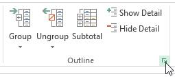
The settings are changed by returning to the Outline section of the Data tab and clicking on the small icon in the bottom right-hand corner (keyboard shortcut, ALT + A + L):

Then, clear both check boxes in the dialog box that appears and then press OK:

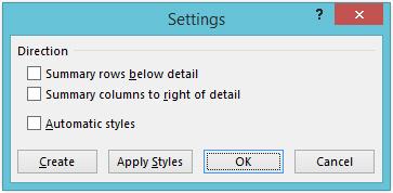
This moves the buttons to the row / column prior to the grouping which, personally, makes more sense to me.

Grouping is very useful in practice. For example, imagine you are a management accountant that has to provide a Gross Profit analysis for your line manager, the Chief Financial Officer and the Board. It is likely that all three stakeholders will require different levels of detail. In the past, I have seen many clients prepare three different spreadsheets for these customers, which causes unnecessary re-work and potential reconciliation issues.

The attached Excel file provides an example of how a [very!] simple solution might look:

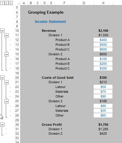
Pressing the numbered buttons will produce all reports required – simple!

Back to the Problem…

So having extolled the virtues of grouping worksheets, I can now return to the reader’s problem: if you protect a worksheet grouping is effectively locked down (i.e. there is no option to enable the various plus, minus and numbered buttons).

So how do we overcome this?

I have explained how to add macros before and to ensure that the workbook is saved as a macro-enabled workbook (please see Locating Links or Automating a Table of Contents for more details).

To protect all sheets, I suggest the following code in the Visual Basic Editor (ALT + F11):

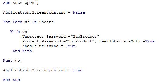
For copying:

When placed in the Auto_Open subroutine, this macro executes upon the file opening (assuming you enable macros). Through the With cycle, it will ensure all worksheets are protected (in this case with the password “SumProduct”) and the command EnableOutlining = True is the code that allows grouping to work. The Application.ScreenUpdating = False and then True later commands freeze the display whilst the code is executed to prevent screen flashing and epileptic fits (this code is employed regularly in many VBA subroutines).

Here at SumProduct, we tend to put this code into all of our final client models as a matter of course: flexibility is the key to a good Excel file.

Word to the Wise

1. Regarding the attached Excel file, I would like to emphasise this file may not work with all versions of Excel. Caveat emptor – it is provided in good faith and should work for most readers. However, I do not have time to enter into correspondence for those unlucky enough to find this file does not appear to work as intended.
2. Make sure you save the workbook as a macro enabled workbook or all will be for nought!