
Power Query: Moving Date
14 March 2018
Welcome to our Power Query blog. This week, I look at how to transform extracted data into a useful table.
Regular readers will be familiar with my fictional salespeople and their tendency to supply data in the wrong format. Let’s meet John.
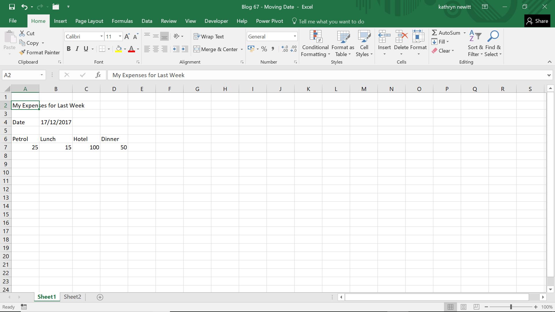
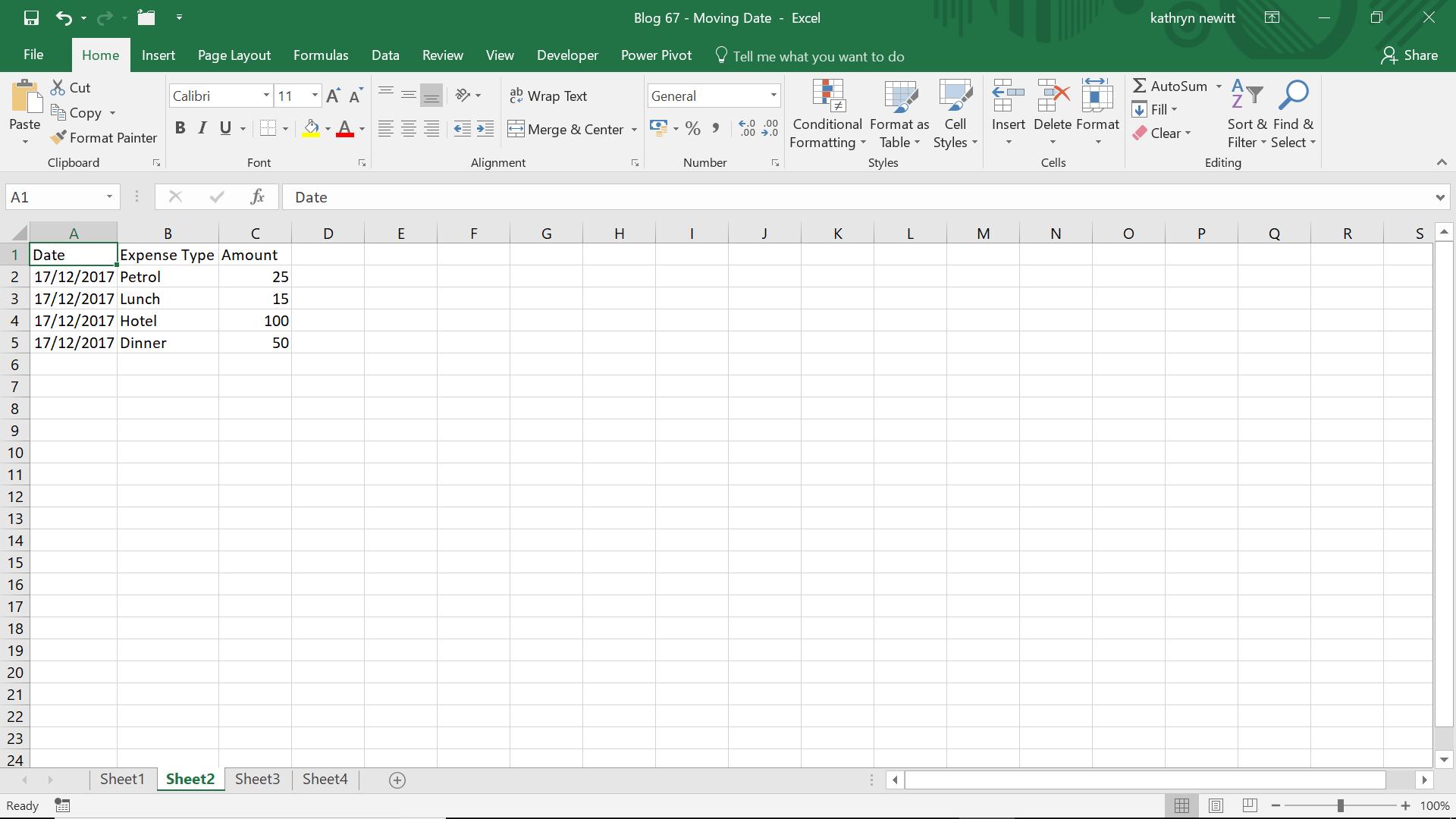
Whilst John has supplied his expenses, the format I would like to see them in is something like this:
To start the process, I extract John’s data into Power Query:
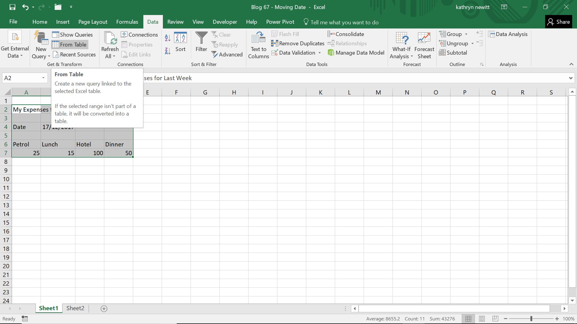
I can select the data and use ‘From Table’ on the ‘Get and Transform’ section of the ‘Data’ tab. My data will be converted to a table as part of the process.
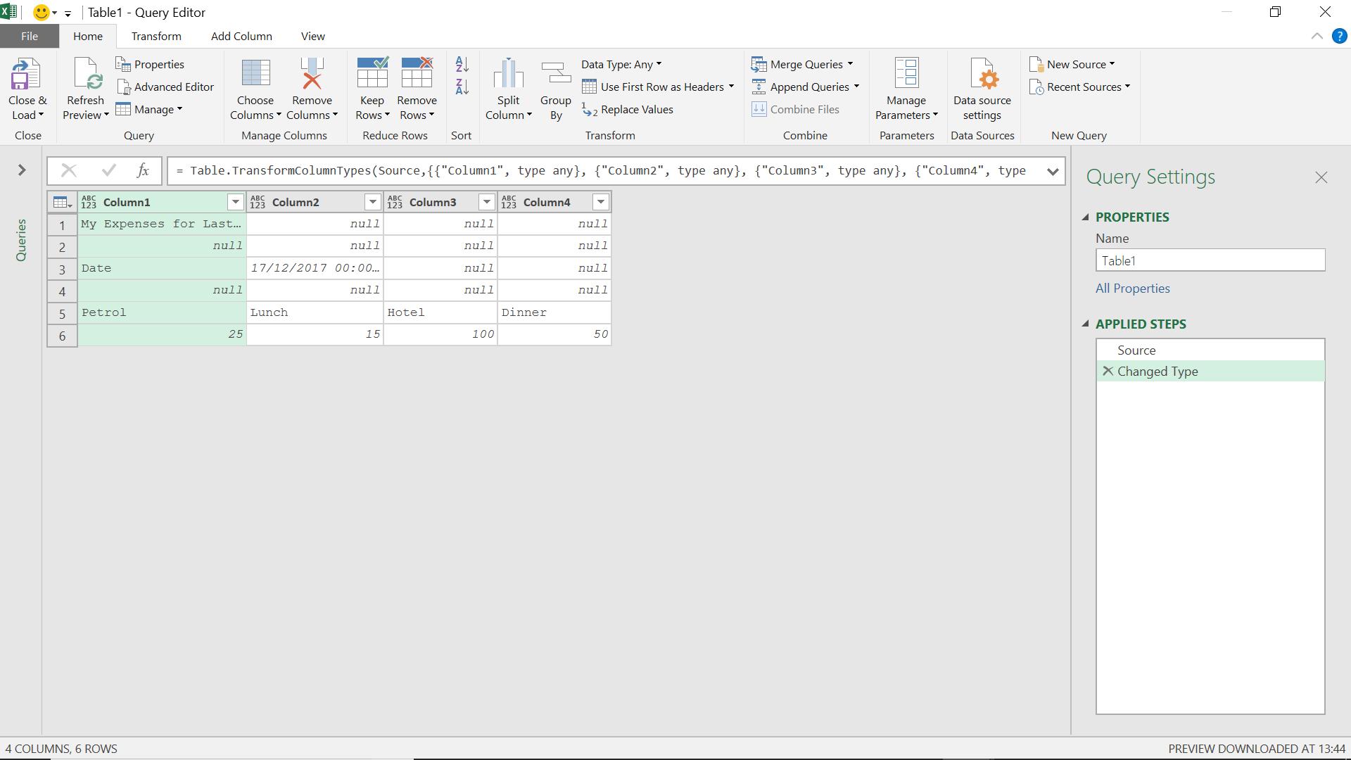
The first two rows are not useful to me, so my first step is to remove them using the ‘Remove Rows’ option in the ‘Reduce Rows’ section.
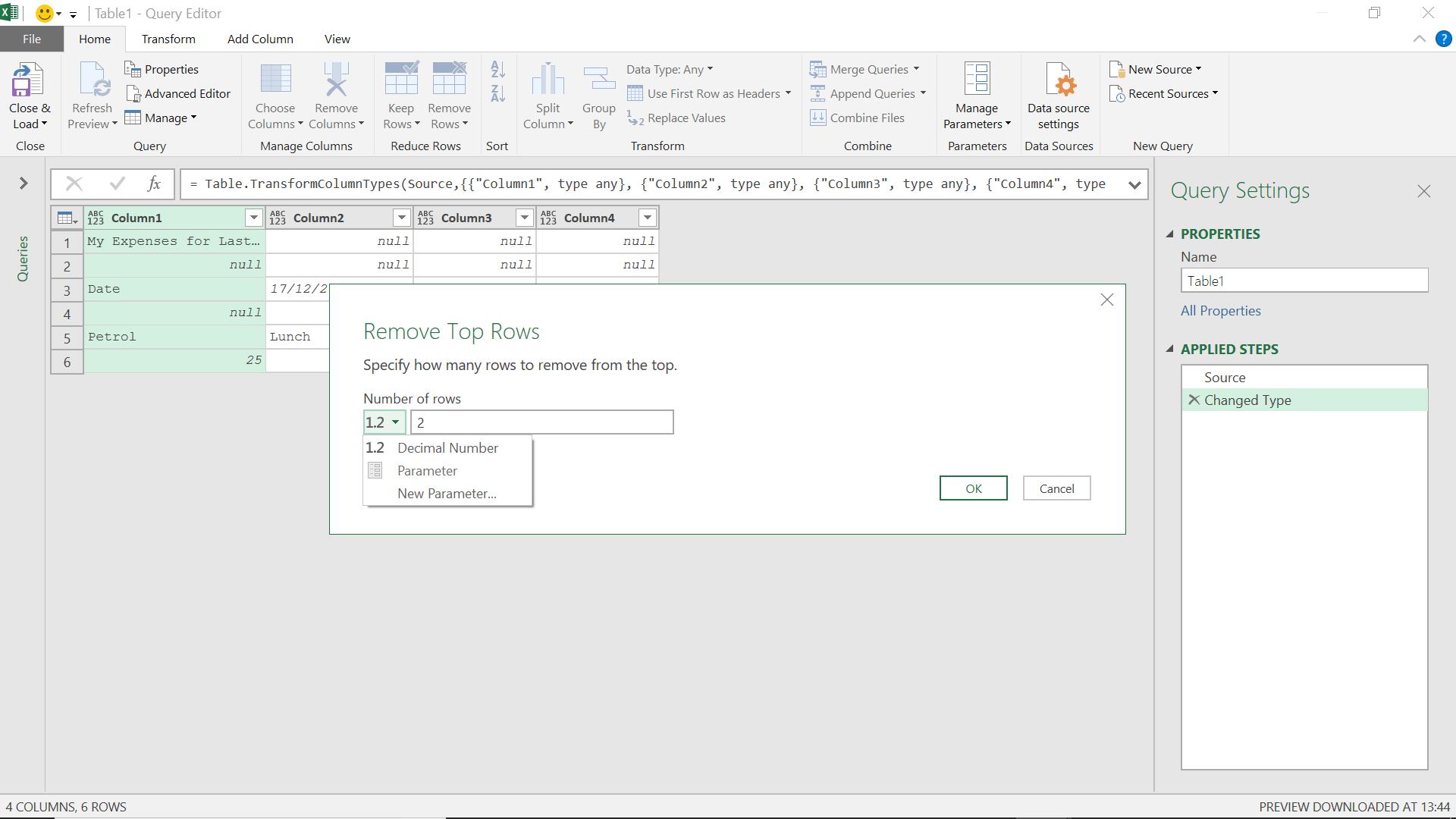
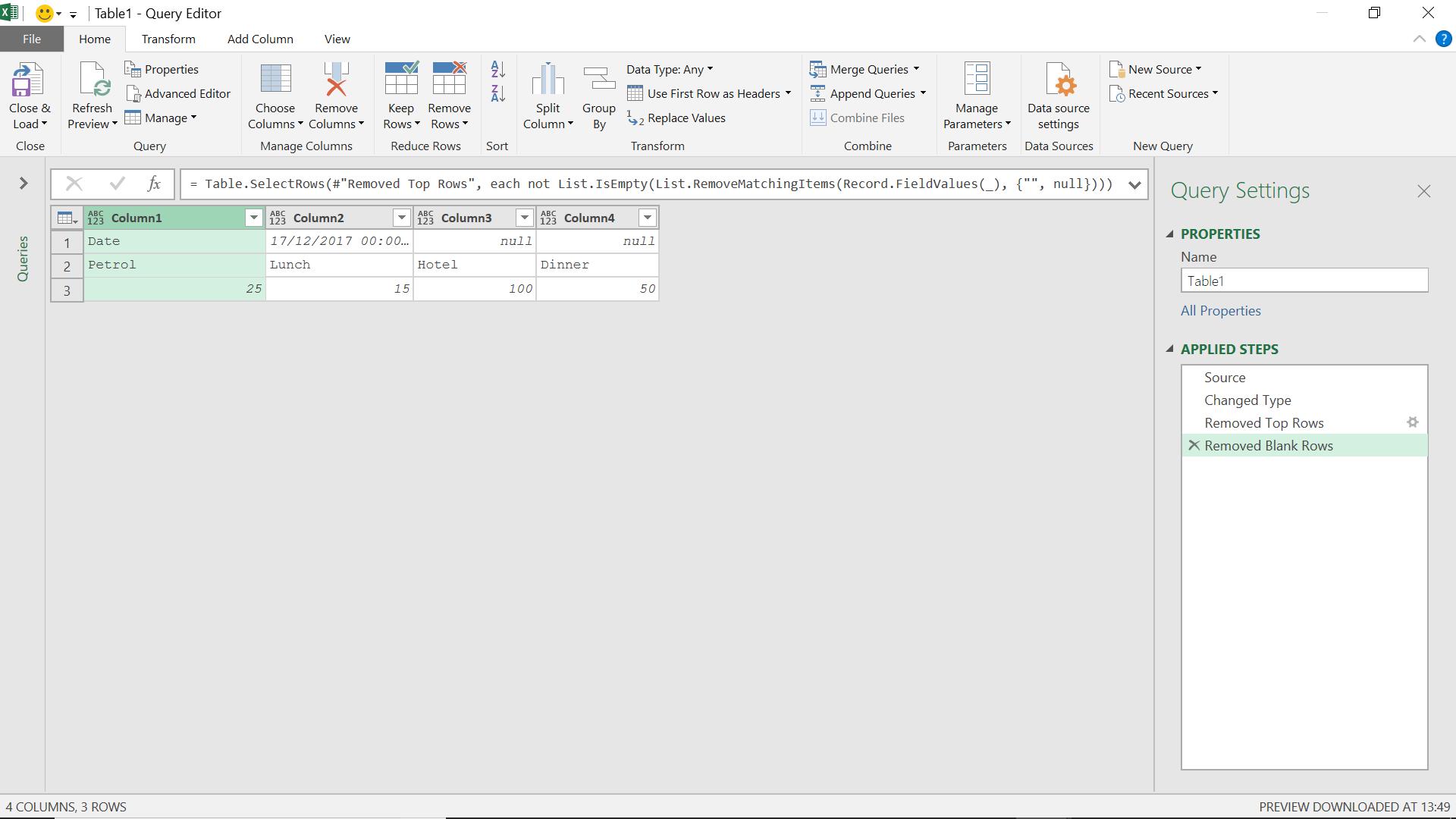
I could remove them based on a parameter, but I just want to get rid of the first two rows so I choose the ‘Decimal Number’ option. I also remove the row of nulls beneath my ‘Date’ row by removing blank rows.
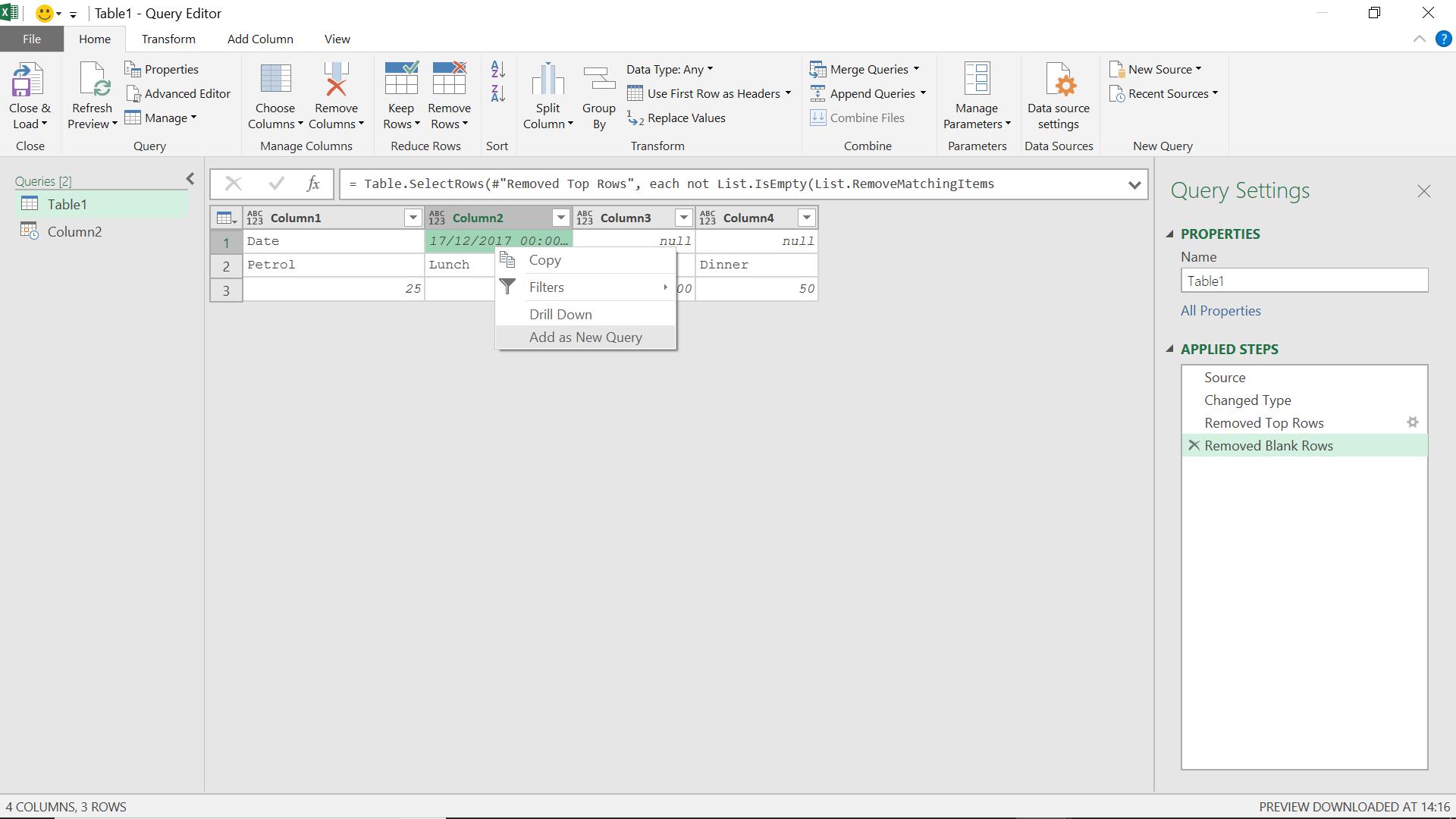
I want to create a column from the 'Date' cell. The first step to achieving this is to right click on the Date cell and use the option to ‘Add as New Query’. This creates a new query in the queries panel on the left of the screen.
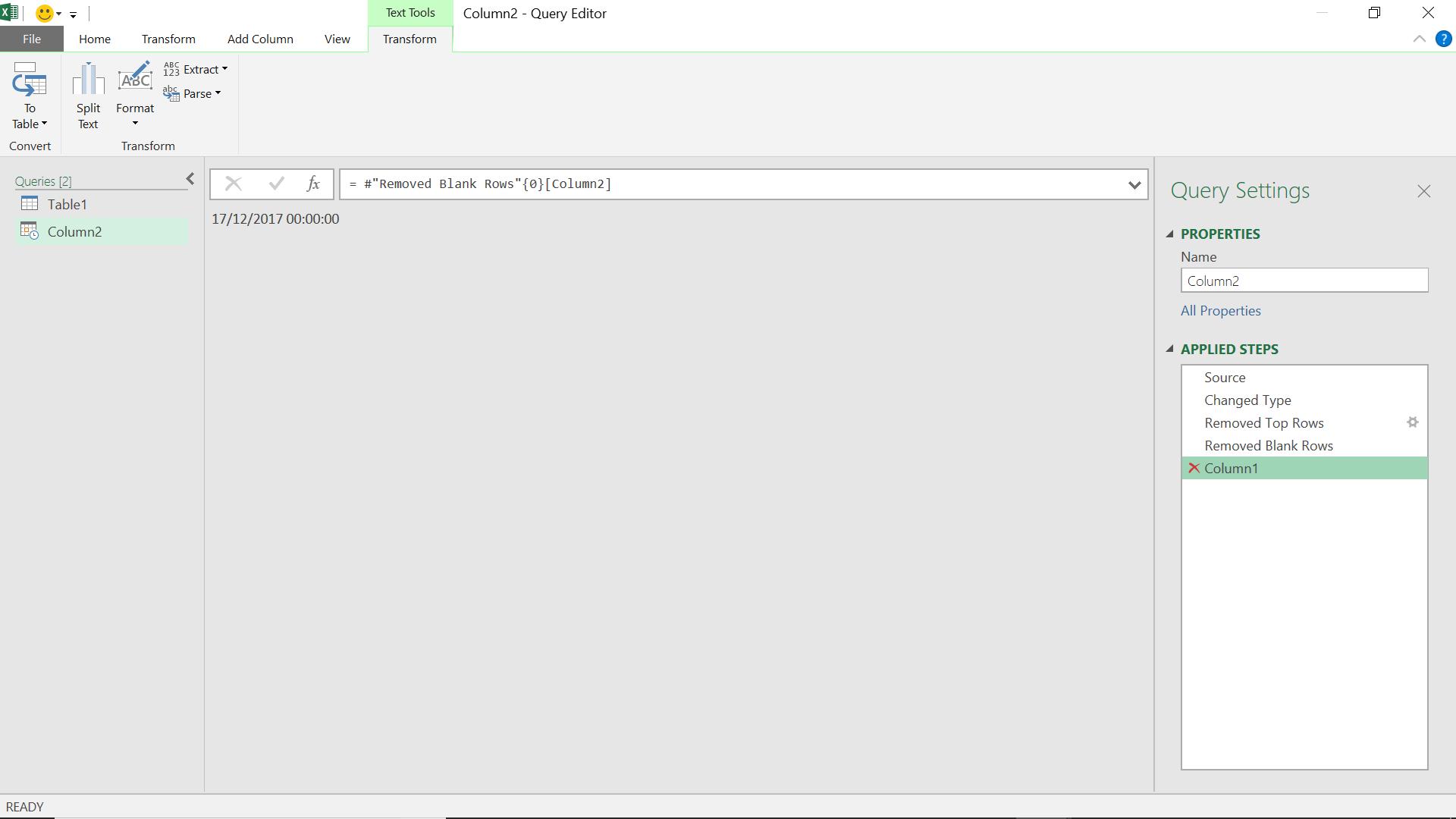
The new query, automatically called ‘Column2’, includes my earlier source steps and the value in the top row of Column2 – the date.
Having created my query, I need to make sure the next steps I add are to the ‘Table1’ query. Now I can transform the rest of the data to appear in the format that I would like.
The steps I have taken are;
- Removed Top Rows1 – having moved the date to a separate query, I could remove the ‘Date’ row
- Promoted Headers – since I wanted to just keep my expense types and values, I promoted the expense to headers to get rid of the generic ‘Column1’ etc. (the ‘Changed Type1’ step was an automated Power Query step)
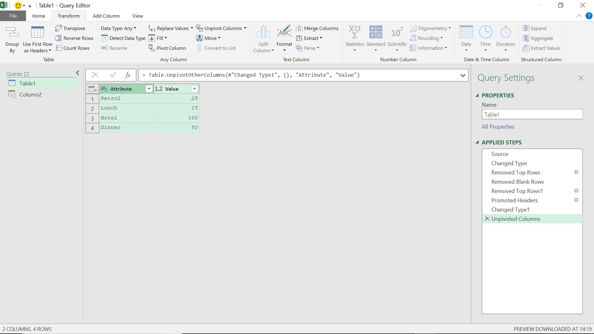
- Unpivoted Columns – I didn’t want to keep my expense types as headers, I ultimately want to store them in a column under the heading ‘Expense Type’, so I unpivoted to get the data as it is shown above.
Now all that remains is to rename my columns and add a ‘Date’ column. To do this I will add a custom column.
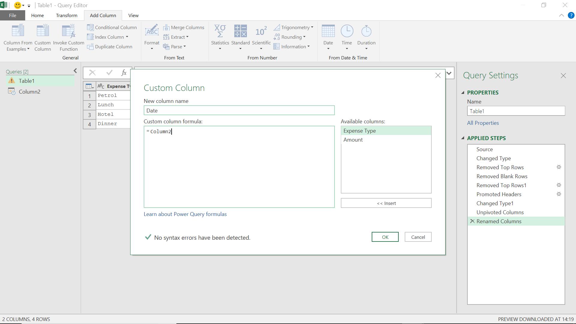
Having referenced the other query (which is easy to check as I can see it in the left-hand pane), I click ‘OK’.
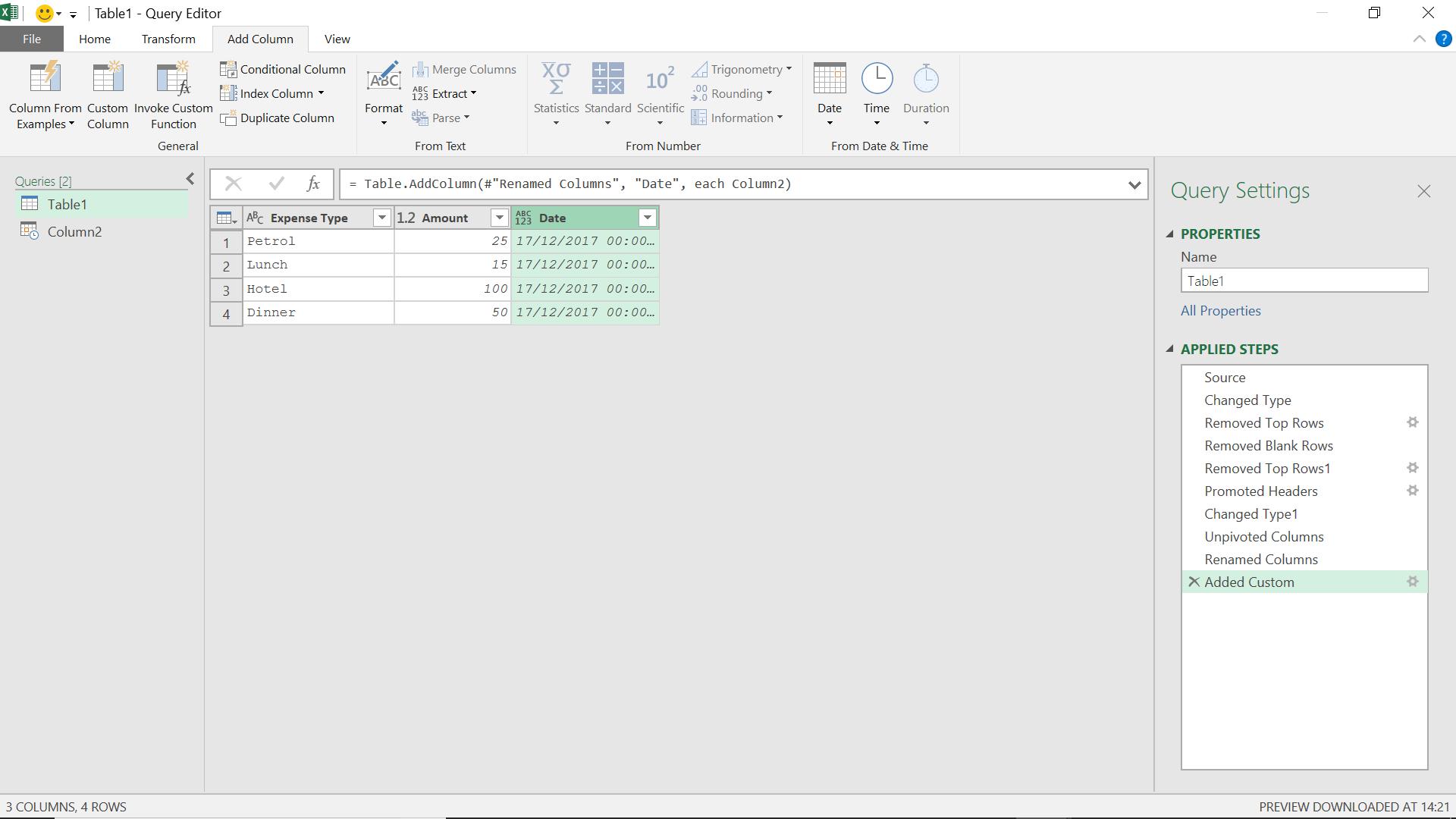
The date appears as a new column.
Want to read more about Power Query? A complete list of all our Power Query blogs can be found here. Come back next time for more ways to use Power Query!