
Power Query: Getting Started
21 December 2016
Our new Power Query blog continues. Today we look at manipulating a simple CSV file
The best way to get to grips with a new tool like Power Query is to start with a simple task. Excel users may often need to take data from CSV (comma separated values) files and transform it ready for analysis. Power Query has been designed to assist with this, so let’s see how easy it can be.
Starting with a new workbook, we open Power Query – the screenshots shown here are from Excel 2013, where Power Query has its own Ribbon, as it does for Excel 2010; for Excel 2016, Power Query is on the Data tab in the ‘Get & Transform’ group. As shown in the last blog, there are a variety of possible sources to extract from in the Get External Data section of the Ribbon.
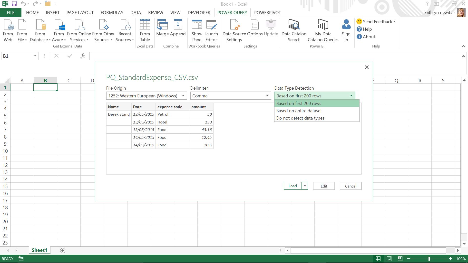
For this example, we are using the ‘From File’ option and browsing to the location of a simple expense CSV file. The image below appears first (this has been added in a recent update, so if you go straight to the Power Query Editor, you are missing the latest update – see the Installing and Updating blog for guidance on this). This intermediate screen has been added to give the user the option to decide whether Power Query should make some assumptions about data types. This will become clearer when the steps are generated so take the default option to allow Power Query to detect data types ‘Based on first 200 rows’ (more than enough for out short example). We could just choose to load from this point, but instead, choose to Edit or transform the data:
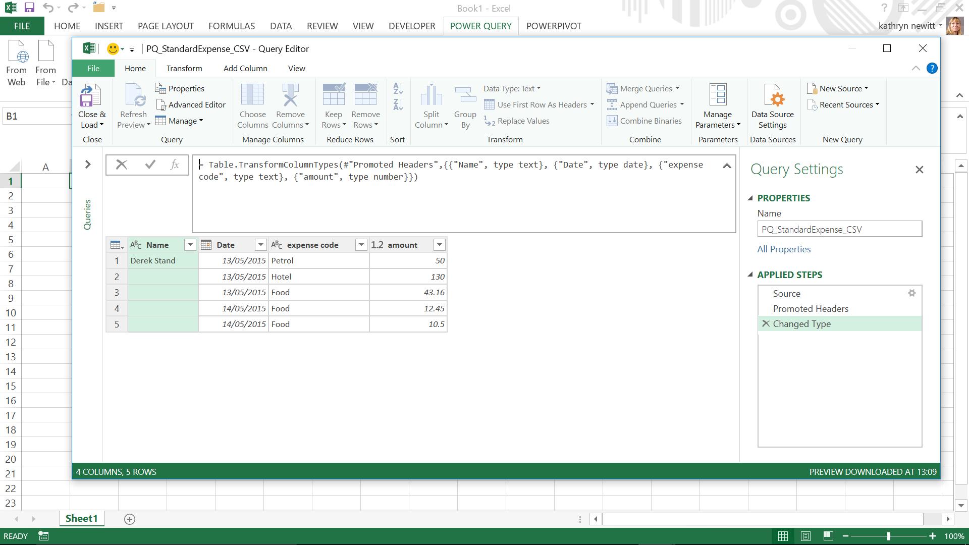
The Power Query Editor screen appears, which shows the table of data as it will be uploaded and the steps that Power Query has taken automatically. The source has been identified, the header column names have been assumed, and as shown in the screen below, the ‘Change Type’ step sets the detected type for each column. The syntax for this is:
=Table.TransformColumnTypes(#"Promoted Headers",{{"Name", type text}, {"Date", type date}, {"expense code", type text}, {"amount", type number}})
This is a simple example of M code, which will be explored in more detail in future blogs. It is essentially a list of column names and their assigned data types based on the data that Power Query has analysed:
- Name is type text
- Date is type date
- expense code is type text
- amount is number.
In this case, all the assumptions look good so we can accept Power Query’s automatic assignment of data types.
We can then make any changes to the data, such as changing column names or removing columns. Selecting a column and viewing the ‘Transform’ tab reveals buttons for many common actions like this. If we choose to rename expense code and amount to Expense Code and Amount, then Power Query not only creates a step, but knows to combine both renames into one step:
= Table.RenameColumns(#"Changed Type",{{"expense code", "Expense Code"}, {"amount", "Amount"}})
A more complex step is to make the Name data appear on each row. In order to use the ‘Fill Down’ button, the Name cells that are to be populated must be set to null and they are currently blank. Therefore, we need to replace the blanks with null and then fill down:
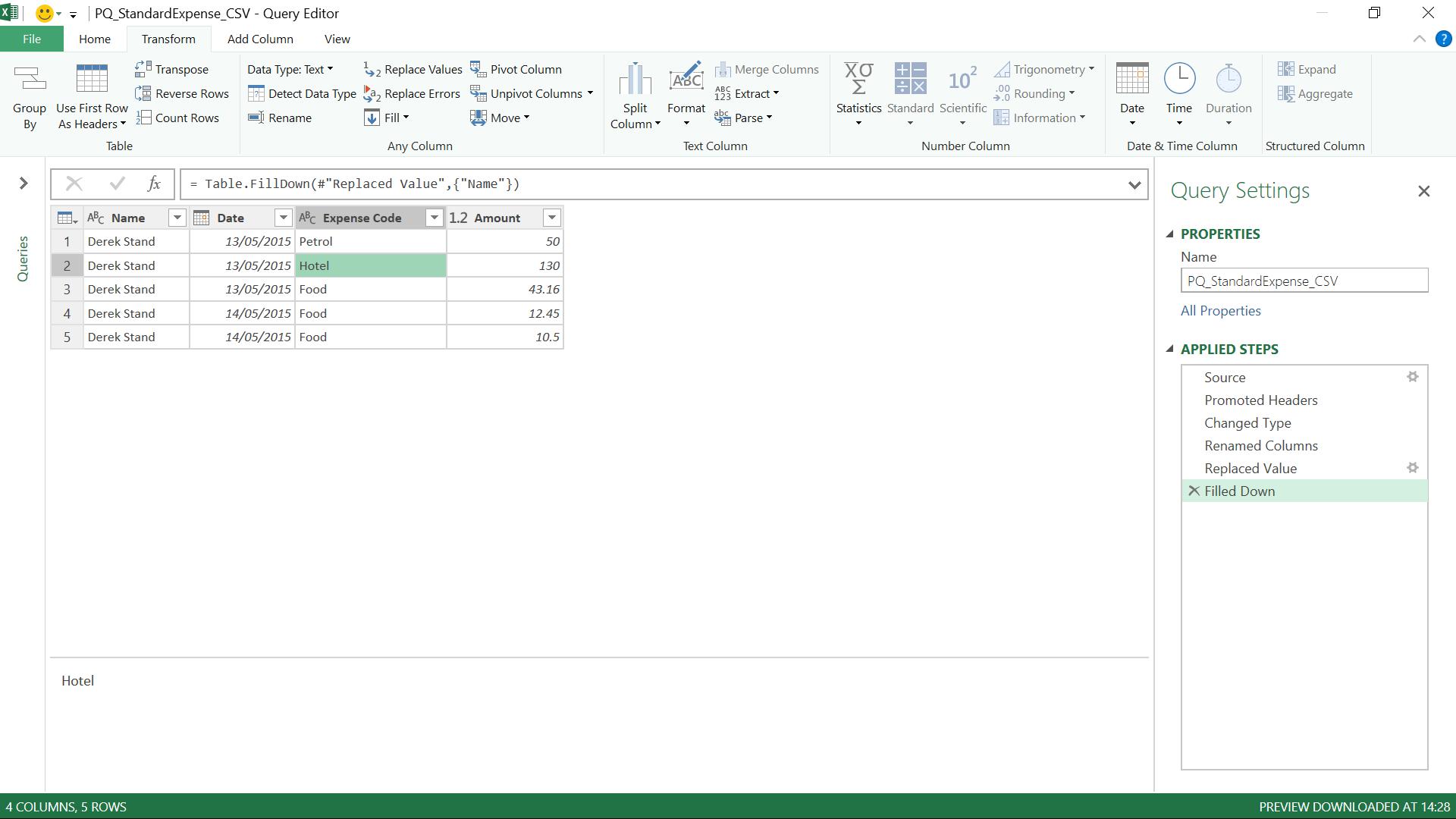
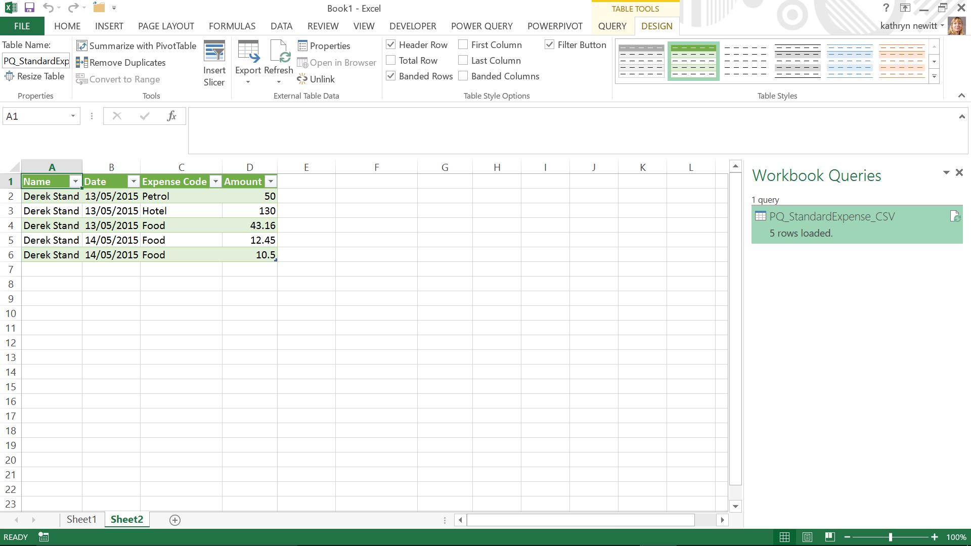
The steps are generated in the right-hand pane, and we are ready to load to Excel using the ‘Close and Load’ button on the ‘File’ tab. The uploaded table is shown below, and the Workbook query window displays the query that generated the data, so that it can be updated and / or refreshed as required. The ‘TABLE TOOLS’ tab opens automatically ready for use in the Excel workbook:
Next time, we’ll look at appending more data…
Want to read more about Power Query? A complete list of all our Power Query blogs can be found here. Come back next time for more ways to use Power Query!