Power Pivot Principles: Power Pivot Menu in Excel

Welcome back to our Power Pivot blog series. To conclude our series covering menu tabs, we will cover the Power Pivot menu options in Excel.

Below is a screenshot of the Power Pivot tab option in Excel:

Power Pivot Menu

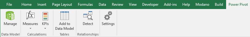
Data Model

This option allows us to access our Power Pivot data model (i.e. where the data is stored “behind the scenes”). We can load and prepare data or continue working on data already added to this workbook.

Calculations

Like we can do in the Power Pivot data model, the ‘Measures’ and the ‘KPIs’ options allow you to add or manage ‘Measures’ and ‘KPIs’.

Tables

‘Add to data model’ will allow us to create a linked table by adding the Excel table to the data model. Linked tables are a live link between the table in Excel and the table in the data model, so updates to the table in Excel automatically update the data in the model. If this table is already in the data model then this action adds a copy to the model.

Relationships

This option will automatically detect and create relationships between tables used on the selected PivotTable.

Settings

This allows you to define settings for your Power Pivot environment and specify language options.

This completes the overview of all of the menu options available in Power Pivot – we will move on next time.

That’s all for this week, stay tuned for our next post on Power Pivot. In the meantime, please remember we have training in Power Pivot which you can find out more about here. If you wish to catch up on past articles in the meantime, you can find all of our Past Power Pivot blogs here.