Power Pivot Principles: Filters Revisited

Welcome back to our Power Pivot blog. Today, we discuss another way to use Filters in Power Pivot.

In a previous blog, Power Pivot Principles: Filters, we discussed how to use Filters in a PivotTable created with Power Pivot. This week, we will discuss how to incorporate filters directly into the measures we create in Power Pivot.

We begin with creating a new table with the following values:

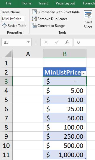
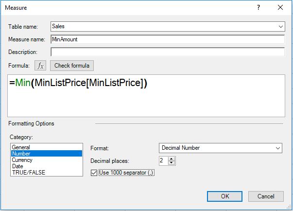
Remember to name the table ‘MinListPrice’.  We will then add this table to our Data Model.  After adding it to our Data Model we can create a new measure called ‘MinAmount’ with the following formula:

Our next move is to create another measure called Sales Above Selected Unit List Price, where the formula should be:

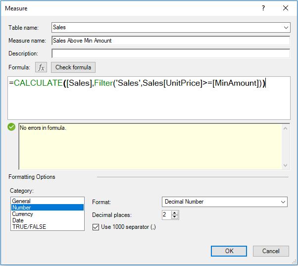
Note that this formula wouldn’t work without using the FILTER function.  This is because the calculation has to be performed on a record by record basis, rather than in aggregate, as CALCULATE usually works.  This requires you to filter records, i.e. use the FILTER function. 

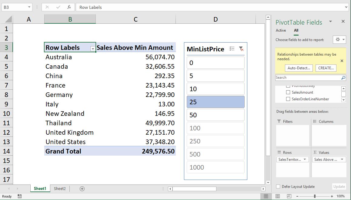
Insert a slicer for MinListPrice and add the Sales Above Min Amount into the ‘Values’ area of the PivotTable.

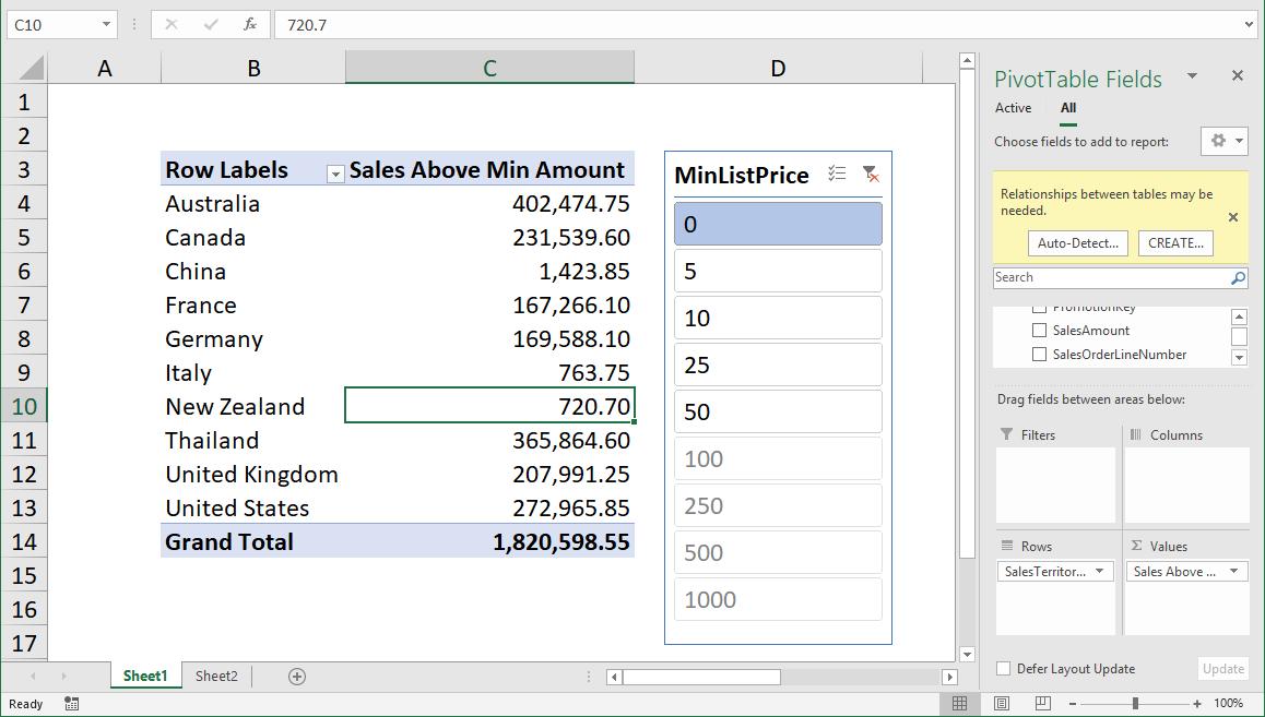
Selecting different price points in the slicer will highlight the amount of Sales made where the unit price is above the minimum price point.

Interesting? We can apply the greater than or even the equals to operator to this filter.

That’s it for this week!

Stay tuned for our next post on Power Pivot in the Blog section. In the meantime, please remember we have training in Power Pivot which you can find out more about here. If you wish to catch up on past articles in the meantime, you can find all of our Past Power Pivot blogs here.