
Power Pivot Principles: Doing More with CALCULATE
29 May 2018
Welcome back to our Power Pivot blog. Today we discuss how to do more with the CALCULATE function.
In Power Pivot we can use the CALCULATE function to filter our total sales amount by the Product Type, Weeks, or Months. You can read more about it here. That blog just covered a single criterion, so let’s extend it – what if we have two criteria that we wish to filter by instead?
In our data here, we have four PromotionKey types: 1, 2, 13, 14. Promotion keys 2 and 14 represent refunds. The aim is to ascertain the total amount of refunds.
The solution is simple:

We simply add two formulas together. However, in another subtly different scenario, what if we only want to sum the refunds if it is classified as promotion key 2 or 14? We could use the OR function:
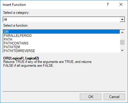
This works like the Excel version of the function. However, there is an alternative which has no Excel equivalent – the OR operator:

The OR operator is two straight lines ‘||’, (you get this by holding down the SHIFT key and pressing the Backslash ‘\’ key twice).
That’s it for this week, stay tuned to our blog for more on Power Pivot. In the meantime, please remember we have training in Power Pivot which you can find out more about here. If you wish to catch up on past articles in the meantime, you can find all of our Past Power Pivot blogs here.