
Power Pivot Principles: Calendar Table
28 August 2018
Welcome back to our Power Pivot blog. Today, we discuss the steps we should take when creating a Calendar Table.
When analysing data, it is important to be able to access past financial information so that comparisons can be made over a time period. To allow us to perform comparisons more easily, we should utilise what is known as a Calendar table. A Calendar table is a date table that links in with the dates in our data. It is vital to have such a table in many types of relational database systems, including Power Pivot.
Before we begin to create our Calendar table there are two important points to remember:
- Ensure that the start date in the Calendar table is before or on the earliest start date in your data model and end on or after the last date in your data model
- Dates must be contiguous (no gaps in days), in ascending order with no duplicates.
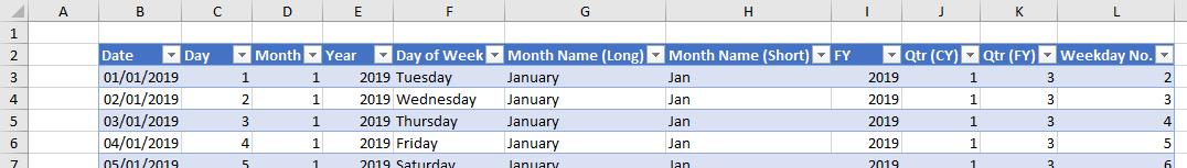
Let’s create our calendar table in Excel, first create the following headings:
- Date
- Day
- Month
- Year
- Day of Week
- Month Name (Long)
- Month Name (Short)
- FY
- Qtr (CY)
- Qtr (FY)
- Weekday No.
Highlight the table headings and convert the range into a Table (CTRL + T):

Name the Table ‘Calendar’ in the ‘Properties’ group of the context-specific ‘Table Tools, Design’ tab of the Ribbon. We can now enter the following formulae under each heading:
- Date: Ensure the start date is before or on the earliest date contained within the data model
- Day: =DAY([@Date])
- Month: =MONTH([@Date])
- Year: =YEAR([@Date])
- Day of Week: =TEXT([@Date],"dddd")
- Month Name (Long): =TEXT(MONTH([@Date]),"MMMM")
- Month Name (Short): =TEXT(MONTH([@Date]),"MMM")
- FY: =YEAR([@Date])+IF(MONTH([@Date])>=7,1,0)
- Qtr (CY): =ROUNDUP([@[Month]]/3,0)
- Qtr (FY): =MOD([@[Qtr (CY)]]-3,4)+1
- Weekday No: =WEEKDAY([@Date],2)
Our Table should be populated now:
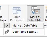
The next step is to add this table to Power Pivot and ensure the table is still called ‘Calendar’.
With the Calendar table highlighted navigate to the ‘Design’ tab and select ‘Mark as Date Table’.
That’s it! Now we have our Calendar table imported into our Power Pivot data model. We may begin to perform time analysis on our data.
More on that next week!
Stay tuned for our next post on Power Pivot in the Blog section. In the meantime, please remember we have training in Power Pivot which you can find out more about here. If you wish to catch up on past articles in the meantime, you can find all of our Past Power Pivot blogs here.