
A to Z of Excel Functions: The CELL Function
24 April 2017
Welcome back to our regular A to Z of Excel Functions blog. Today we look at the CELL function.
The CELL function
With our A t Z of Excel Functions series, you could argue we have been trying to make a soft CELL (get it?). We are well and truly in the high C’s now and the puns do not get any better. Ah well…
The CELL function returns information about the formatting, location, or contents of a cell. For example, if you want to verify that a cell contains a numeric value instead of text before you perform a calculation on it, you can use the following formula:
=IF(CELL("type", A1) = "v", A1 * 2, 0)
This formula calculates A1*2 only if cell A1 contains a numeric value, and returns 0 if A1 contains text or is blank. The CELL function employs the following syntax to operate:
CELL(info_type, [reference])
The CELL function has the following arguments:
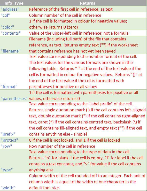
- Info_type: this is required. This is a text value that specifies what type of cell information you want to return. The following list shows the possible values of the Info_type argument and the corresponding results:
- reference: this is optional. This is the cell that you want information about. If this argument is omitted, the information specified in the Info_type argument is returned for the last cell that was changed. If the reference argument is a range of cells, the CELL function returns the information for only the upper left cell of the range.
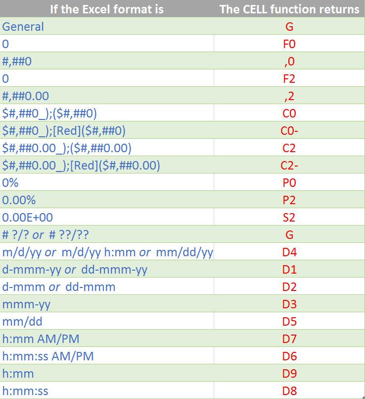
CELL Format Codes
The following list describes the text values that the CELL function returns when the Info_type argument is "format" and the reference argument is a cell that is formatted with a built-in number format.
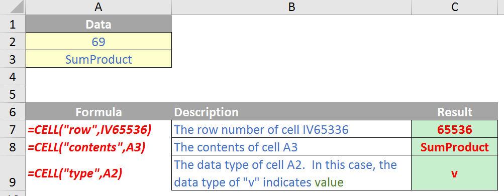
Please see my example below:
There’s lots you can do with CELL. You may recall in one of our Thought articles we used it to automate the file name using the formula
=IF(ISERROR(OR(FIND("[",CELL("filename",A1)),FIND("]",CELL("filename",A1)))),"",MID(CELL("filename",A1),FIND("[",CELL("filename",A1))+1,FIND("]",CELL("filename",A1))-FIND("[",CELL("filename",A1))-1))
You can read up on how this formula works by visiting the relevant article here.