
A to Z of Excel Functions: The AMORLINC Function
27 July 2016
Welcome back to our regular A to Z of Excel Functions blog. Today we look at the AMORLINC function.
The AMORLINC function
The AMORLINC function in Microsoft Excel is similar to the last function we discussed, AMORDEGRC. The difference is that this function returns the depreciation for each accounting period, as provided for the French accounting system. If an asset is purchased in the middle of the accounting period, the pro-rated depreciation is taken into account instead.
AMORLINC uses the following syntax:
AMORLINC(cost, date_purchased, first_period, salvage, period, rate, [basis])
Important: Dates should be entered by using the DATE function, or as results of other formulas or functions. For example, use DATE(2016,5, 23) for the 23rd day of May, 2016. Problems can occur if dates are entered as text.
The AMORLINC function syntax has the following arguments:
- cost: this is required. This represents the cost of the asset
- date_purchased: also required. The date of the purchase of the asset
- first_period: required. The date of the end of the first period
- salvage: required. The salvage value at the end of the life of the asset
- period: required. The period in question
- rate: required. The rate of depreciation
- basis: optional. The year basis to be used.
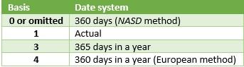
Some notes to remember on how the basis argument works (there’s no number 2):
Also note:
- Microsoft Excel stores dates as sequential serial numbers so they can be used in calculations. By default, January 1, 1900 is serial number 1, and January 1, 2008 is serial number 39448 because it is 39,448 days after January 1, 1900.
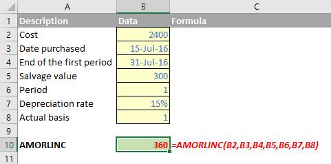
Please see my example below:
We’ll continue our A to Z of Excel Functions soon. Keep checking back – there’s a new blog post at least every other business day.